WIXLIB

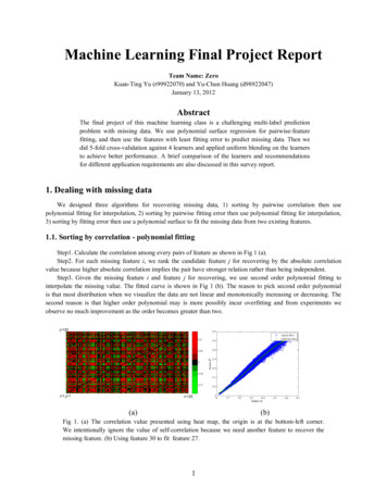
Machine Learning Final Project ReportTeam Name: ZeroKuan-Ting Yu (r99922070) and Yu-Chun Huang (d98922047)January 13, 2012AbstractThe final project of this machine learning class is a challenging multi-label predictionproblem with missing data. We use polynomial surface regression for pairwise-featurefitting, and then use the features with least fitting error to predict missing data. Then wedid 5-fold cross-validation against 4 learners and applied uniform blending on the learnersto achieve better performance. A brief comparison of the learners and recommendationsfor different application requirements are also discussed in this survey report.1. Dealing with missing dataWe designed three algorithms for recovering missing data, 1) sorting by pairwise correlation then usepolynomial fitting for interpolation, 2) sorting by pairwise fitting error then use polynomial fitting for interpolation,3) sorting by fitting error then use a polynomial surface to fit the missing data from two existing features.1.1. Sorting by correlation - polynomial fittingStep1. Calculate the correlation among every pairs of feature as shown in Fig 1 (a).Step2. For each missing feature i, we rank the candidate feature j for recovering by the absolute correlationvalue because higher absolute correlation implies the pair have stronger relation rather than being independent.Step3. Given the missing feature i and feature j for recovering, we use second order polynomial fitting tointerpolate the missing value. The fitted curve is shown in Fig 1 (b). The reason to pick second order polynomialis that most distribution when we visualize the data are not linear and monotonically increasing or decreasing. Thesecond reason is that higher order polynomial may is more possibly incur overfitting and from experiments weobserve no much improvement as the order becomes greater than two.(a)(b)Fig 1. (a) The correlation value presented using heat map, the origin is at the bottom-left corner.We intentionally ignore the value of self-correlation because we need another feature to recover themissing feature. (b) Using feature 30 to fit feature 27.1

1.2. Sorting by fitting error - polynomial fittingAlthough correlation is one heuristic that estimate which two pair has better fitting result, a more directmeasurement would be the fitting error. The fitting error correspond to the training error taught in class. We canfurther use cross validation to further estimate the testing error. As a result we gain a significant improvement intesting performance of the entire multilabel problem. The error we used is root mean squared error (RMSE).1.3. Sorting by fitting error - surface fittingThe method above is good enough for certain feature but not for all features. For example, the best curve to fitfeature 60 is shown in Fig 2. We can observe a great error on the right hand side. Therefore, we propose to use twofeatures to fit the target missing feature in order to lower the fitting error. We can achieve a better fitting error of0.052 against the error of 0.08 obtained from section 1.2. We choose the two features for each target by fitting error.Fig 2. (a) Curve fitting result of feature 60 against feature 56. (b) Surface fitting result.Fig 3. (a) We added some missing value to the testing data to test our recovering mechanism. Thisshows the distribution of L1 error. The error is mostly bounded by 0.1.2. Choosing learnersIn order to find a good multi-label predictor for this particular data set, we applied 5-fold cross-validationagainst 4 learners (MLkNN, J48, SVM, and Random Forest1) with various parameter configurations. Note that, allthe parameters not listed here are left using implementation defaults. After the evaluation is done, uniform blendingis applied to further improve the performance.1We applied two meta-algorithms (RAkEL and Power Labelset[3]) to J48 and Random Forest.2

The learner implementations we use for this project are Mulan[1] and LIBSVM[2]. The source code of thisproject can be found at . MLkNN 5-fold cross-validationTable 1. MLkNN 5-fold cross-validation resultKSmoothnessHamming lossF180.70.0328 0.00030.4844 0.001881.00.0328 0.00030.4844 0.001881.30.0328 0.00030.4844 0.0018120.70.0326 0.00030.4829 0.0023121.00.0326 0.00030.4828 0.0023121.30.0326 0.00030.4828 0.0023160.70.0325 0.00030.4849 0.0039161.00.0325 0.00030.4849 0.0039161.30.0325 0.00030.4849 0.0039221.00.0324 0.00030.4904 0.0046261.00.0323 0.00030.4909 0.0030301.00.0323 0.00030.4895 0.002534*1.00.0323 0.00030.4922 0.0034* Considered the best choice and used by our team.2.2. J48 5-fold cross-validationTable 2. J48 5-fold cross-validation resultConfidence intervalHamming lossF10.250.0321 0.00020.5572 0.00360.30*0.0322 0.00020.5569 0.00360.400.0322 0.00020.5569 0.00370.500.0323 0.00020.5569 0.0038* Considered the best choice and used by our team.3

2.3. Random Forest 5-fold cross-validationTable 3. Random Forest 5-fold cross-validation resultNumber of treesNumber of featuresHamming lossF11030.0287 0.00020.5659 0.00291050.0285 0.00030.5716 0.00171080.0261 0.00010.6192 0.002110120.0262 0.00010.6194 0.004010160.0261 0.00020.6201 0.002310200.0261 0.00020.6216 0.00372080.0255 0.00020.6264 0.003420160.0254 0.00010.6296 0.002820240.0253 0.00020.6317 0.002920*320.0253 0.00010.6320 0.002420400.0254 0.00020.6316 0.00293080.0255 0.00020.6259 0.003630160.0253 0.00020.6292 0.004330240.0253 0.00020.6304 0.003130320.0253 0.00020.6318 0.0033* Considered the best choice and used by our team.2.4. SVM 5-fold cross-validationWe tried two meta-algorithms to transform the multilabel problem into single label classification problem, 1)label combination 2) binary transformation. For label combination method, we obtain 3436 classes from all possiblelabel combination in the training dataset. However, the best result we obtained is (Hamming loss: 3.7092 F1:0.5284515637) using surface fitting data, which is very limited. The reason we think is because after dividing all thedata into 3436 classes, there are not much examples left for each class, and the number of examples of each class isunbalanced.For binary transformation, we obtain generally better result than using label combination but the training time israther long, because every label requires both training and testing. On the other hand, the default of libsvm outputsaccuracy, which is correspond to hamming loss. To optimize the parameter for F1 score, we modify the output to beF1 score so that the “grid.py” program for choosing SVM parameters that will maximize the F1 score.Table 4. SVM 5-fold cross-validation result4

Recover methodHamming lossF1SVM BinarySurface fitting3.0470.5734046426SVM BinaryErrSort CurveFitting3.26040.5163759345SVM BinaryCorrSort CurveFitting3.5980.4434131551SVM Label CombineSurface fitting3.70920.5284515637SVM Label CombineErrSort CurveFitting3.78860.5387293934SVM Label CombineCorrSort CurveFitting4.23940.40778923252.5 BlendingWe tried 3 methods for blending, 1) Pocket PLA, 2) Linear Regression, and 3) Uniform voting. After severalexperiments, we found that uniform blending generates best result and is much simpler. Hence we use uniformblending to produce the final prediction for the test data set.We also tried several prediction combinations of the 4 learners to do uniform blending. Interestingly, the resultshows that mixing MLkNN and J48 altogether with Hamming-optimized SVM, F1-optimized SVM and RandomForest does not help. We believe the reason why MLkNN and J48 does not make the prediction better is thatRandom Forest and the 2 SVMs are already too powerful, and the votes from MLkNN and J48 are not accurate.Therefore, blending Hamming-optimized SVM, F1-optimized SVM, and Random Forest is our final choice, andit does help us win the 3rd place in turns of Hamming loss in the final competition (Hamming loss: 2.9942; F1:0.5802797948).3. DiscussionIn this section, a brief comparison of the 4 learners, and recommendation for different application requirementsare discussed.Because our team’s best Hamming loss and F1 are predicted by our blending solution, we recommend thisblending solution for both Hamming loss and F1. The pros and cons are also stated in Table 6 (applicationrequirement: “Hamming loss is important” and “F1 is important”).Table 5. Comparison between the 4 HighRandom ForestMediumMediumHighHighSVMLowMediumHighLowTable 6. Recommendations for different application requirements5

ApplicationRequirementComputation time iscriticalOut-of-sample erroris critical(Hamming loss &F1)Recommendation*Pros and cons**MLkNNPros:- Fast (train: 16.74 minutes; predict: 14.64 minutes).Cons:- Comparing to other learners evaluated by us, theout-of-sample error is relatively high for bothHamming loss and F1.Uniform blending of RandomForest and SVMPros:- Out-of-sample error is low, especially forHamming loss measure (Hamming loss:0.029942; F1: 0.5802797948).Cons:- Computation intensive (training time is more than24 hours).- Hard to interpret how the prediction is done.Decision maker should have “faith” on thelearner.Hamming loss iscriticalSame as aboveSame as aboveF1 is criticalSame as aboveSame as above* Learner configurations are based on the cross-validation results discussed in section 2.** Computation time is machine-dependent.4. CreditsKuan-ting Yu (r99922070)- Missing data pre-processing;- SVM prediction;- Survey report.Yu-chun Huang (d98922047)- MLkNN, J48, and Random Forest prediction;- Prediction blending;- Survey report.References[1] Mulan: A Java library for multi-label learning, http://mulan.sourceforge.net/.[2] LIBSVM -- A Library for Support Vector Machines, http://www.csie.ntu.edu.tw/ cjlin/libsvm/.[3] Multi-Label Classification: An Overview, International Journal of Data Warehousing & Mining, 3(3), 1-13, JulySeptember 2007.6

Machine Learning Final Project Report Team Name: Zero Kuan-Ting Yu (r99922070) and Yu-Chun Huang (d98922047) January 13, 2012 Abstract The final project of this machine learning class is a challenging multi-label prediction problem with missing data. We use polynomial surface regression for pairwise-feature