Transcription
Session 73L, Advanced Analytics and Predictive Modeling in LossReservingPresenters:Mark M. Zanecki, ASA, MAAASOA Antitrust DisclaimerSOA Presentation Disclaimer
SSession: 73“actuarial‘reservebots’ ”Advanced Analytics andPredictive Modeling in LossReserving – First GenerationMachine LearningAuthor:Mark Zanecki ASA, MAAASOA Antitrust DisclaimerSOA Presentation Disclaimer2018 SOA Health SeminarAustin, TexasJune 25-27IHA Consultants Inc.
Agenda Introduction Overview of State of the Art Machine Learning Results (Exec. Summary) Survey of Audience Predictive Analytics Framework Overview of Current Modeling Techniques Theory Application Results Demo Summary Questions“actuarial‘reservebots,’ yousay ”Data Science Department – ‘We’re working on it ’Credit: IHA Consultants Inc. Credit: Microsoft Credit: Mystery Science 30002 Satellite of Love, LLC 2017IHA Consultants Inc.
To Participate, look for Polls in the SOA Event App or visit health.cnf.ioin your browserFind The Polls FeatureUnder More In The EventType health.cnf.io In YourAppBrowserChoose yoursessionor3IHA Consultants Inc.3
4IHA Consultants Inc.
5IHA Consultants Inc.
6IHA Consultants Inc.
7IHA Consultants Inc.
8IHA Consultants Inc.
Do you knowwhere youare in yourdistribution?At 25,000 foot Level – we have ‘CVM’:There are three modeling camps: “(Cents) -Centralists” – filter(smooth) results to removefluctuations and rely on central limit theorem (CLT). Pointestimate technique. Actuaries and econometricians favor thiscamp. “(Vols) - volatility” – model volatility ( tame volatility andresults follow by CLT in distribution form. Some actuaries , agood number of econometricians, many statisticians and everyinvestment bank stock options quant. “(MLs) -Machine Learning” – using historical data developmodels using as many predictor variables (called features) asrequired combined with varying correlation and partitioningmethodologies. Membership is open if you know computeralgorithms, computer technology, data considerations,statistics, mathematics, econometrics and enjoy “challenges.”Caution: Finding local optima and not global optima is notalways acceptable nor sufficient. (‘no second best suffices.’)9You arehere.andalso here.IHA Consultants Inc.
Theory, Application and Results Learned (Exec. Summary):Theory: Regression defines error as:error realized value – predicted value(via model) Machine Learning partitions error as:𝑒𝑒𝑒𝑒𝑒𝑒𝑒𝑒𝑒𝑒 𝑏𝑏𝑏𝑏𝑏𝑏𝑏𝑏 ��𝑣𝑣𝑣 You can do better, using the following extension:𝑒𝑒𝑒𝑒𝑒𝑒𝑒𝑒𝑒𝑒 𝑏𝑏𝑏𝑏𝑏𝑏𝑏𝑏 𝑠𝑠𝑠𝑠𝑠𝑠𝑠𝑠𝑠𝑠𝑠𝑠 ��𝑣𝑣𝑣 Application: The ideal machine learning “factory” relies on automation in the following sense(s):a) continuous re-training of existing models on new data,b) has the capability of creating new models when old models are insufficient ( alsopart of the automation process.) The challenge is to create this capability. Successful machine learning automation frameworks rely on many layers beginningwith data and proceeding to many layers of modeling. The ability to detect and quickly recover from algorithmic error or data error is critical. Machine learning requires high compute speed, vast memory size, very high storagesize ( Tera/Peta scale) which is delivered via gpu compute environment at the high endand via Hadoop type at the lower end. Driving firm value from data science requires more than just staffing a department,purchasing off-the-shelf-software and running large amounts of data thru models.10IHA Consultants Inc.
Theory, Application and Results Learned (Exec. Summarycontinued):Result(s): Saving the Best for Last – US Stock Price Prediction Analysis: Using machine learningbased upon gpu servers; 8,500 stock symbols are scanned and next day trading rangeis predicted with accuracy greater thanbased upon prior 20 trade day analysis. Is there a similar result for loss reserves? Ans: Yes, and it is “No risk no reward was verified.” The best stock(s) reported alpha at no greater thanzero, none reported alpha 0 and majority had alpha 0, for short duration horizons.Upward trend /downward trend was attributable toandImplication: The “winner” will be those firms that can measure, model andprice/package volatility ( e.g. embrace it ) – the future for pure smoothing is limited bycomparison. Announcement(s): The audience is encouraged to use the interactive session evaluation app. There is finally a useful app for my Windows Smartphone (stock price predictionapp) that actually uses Mobile Excel. Who would have expected to have to write ityourself?11IHA Consultants Inc.
Why do you need a Machine Learning Factory ( automation)?(data,timeline)First iteration – data,model estimationmodel1model2model3 .model(n)Second iteration – data,model estimationmodel1model2model3 .model(n)Comparing modelingepochs:1) can have samemodel withdifferentparametersOR2) new model withdifferentparameters.Modeling must check all models and then via automation pick optimal model.You need GPU server(s) to do this .12IHA Consultants Inc.
Predictive Analytics / Machine Learning - Audience SurveyTBD – show of hands.13IHA Consultants Inc.
14IHA Consultants Inc.
15IHA Consultants Inc.
16IHA Consultants Inc.
Predictive Analytics / Machine Learning Framework:There are three levels of predictive modeling.Level 1:Analytical methods (descriptive statistics) that are based on summarizing historical datastored in data lake / date warehouse. Typically use Tableau for visualization in combinationwith a business intelligence tool.Level 2:Predictive Modeling which focuses on identifying, classifying and quantifying variousrelationships learned from past data using supervised learning and unsupervised learningtechniques. Model(s) are then used to predict various outcomes. Base model is some formof logistic modeling. More advanced forms include ensemble modeling ( bias reduction),decision trees, gradient boosted methods (GBM), structured vector machines (SVM), andnumerous forms of artificial neural net models (ANN).Level 3:Prescriptive Modeling which focuses on first identifying members in a population based onpredictive modeling results and then forming an action or recommendation as a secondstep.17IHA Consultants Inc.
Overview of Current Modeling Techniques ( next 8 slides ):Reserving as Predictive Problemvs.Regression as Machine Learning Problem Model ConsiderationsData ConsiderationsAssumption ConsiderationsSLA - Time to remental Lossor Cumulativeloss6,000201417,000201425,000201507,000 20171?20180?IHA Consultants Inc.
Loss Reserve as Linear Regression ProblemyXCYDurCumulative loss201406,000201417,000201425,000201507,000 20171?20180?The Regression Problem:𝑆𝑆𝑆𝑆𝑆𝑆𝑆𝑆𝑆𝑆 𝐗𝐗𝐗𝐗 𝐲𝐲 19where X is design matrix𝐲𝐲 is response vector variableRequires error assumption – Normal istypical.Assumes homoscedastic error,independence of columns and otherassumptions. (CF violates thisassumption. Determinant is close to0.0)Using linear predictors in non-linearsituations has unacceptable error rate.IHA Consultants Inc.
Example of a random sequencewith bunching towards mean 0with initial low volatility thatincreases over time.Stochastic Time Series1111111111tennis ball servertimeFigure - as viewed from wall and overhead camerasIllustrative models include: Moving Average Auto-regressive ARIMA – combination of moving average & auto-regressive More sophisticated: GARCH which involves modeling time varying volatility(various flavors). This requires solving Maximizes Log of Likelihood functionwhich is a non linear optimization problem. Mean-reversion processes only.20IHA Consultants Inc.
SimulationCDF Simulation is useful to estimate the predicted distribution ofvalues generated by numerous path iterations. In life insurance reserving, simulation is the tool for valuationfor secondary guarantee reserves. Healthcare loss reserves use simulation to develop bestestimate or to estimate variability of best estimate.21DurationIHA Consultants Inc.
Generalized Linear Model 38125415015516052002106222CYDurIncremental t(s): Error distribution:Tweedie/Gamma/Poisson 20171?Predictors: Calendar year,duration/development period, etc. 20180?Results sensitive to errorassumption. Available in Python, R, Matlab,SAS and other packagesYCY, Dur exp(β0 βCY βDur) εLog 30 123.5121 115116 110120 114106 100132Linear combination of explanatory variables predicts incrementallosses, based on CY and Dur and other identified predictors.IHA Consultants Inc.
Theory: Machine Learning (Supervised)No limit to number of features. Discovery of smallest, reliable feature set is the problem.“Train model” using historic data features and apply to future data predictors.To each 𝒀𝒀𝒊𝒊 associate a function of 𝑋𝑋 variables. ( This is trial and error process. )CYDur2014201420142015 201720180120 10𝐗𝐗Var 1 Var 2 Var 3 yIncremental Lossor Cumulativeloss6,0007,0005,0007,000 ?New Predictors23IHA Consultants Inc.
Theory: Machine Learning (Supervised) – Thought Experiment(s)As X variables vary, 𝒀𝒀𝒊𝒊 varies – static model learned from historic data for that period.What happens if over time, 𝒀𝒀𝒊𝒊 varies not only with X variables but also by passage of time? Ans: frequemt retraining. (Recurrent Neural Net is typically used.)What is one of the fundamental differences between machine learning vs classical regression? Ans: From linearalgebra the column space must be full span, non-zero determinant, independent and ideally non correlated. Notforgetting heteroscedasticity.CYDur2014201420142015 201720180120 10𝐗𝐗Var 1 Var 2 Var 3 yIncremental Lossor Cumulativeloss6,0007,0005,0007,000 ?New Predictors24IHA Consultants Inc.
Machine Learning (Supervised) – Thought ExperimentConsider for claim type (hospital inpat., outpatient; physician inpat., outpat, office , drug etc.) modeling by durationusing claim amount bins and claim count.What are the pros & cons? Ans: Reduces problem to Poisson Count (by claim detail type and by bin) but withpopulation origination, timing and trend considerations.y𝐗𝐗Duration 0 Claim Amount Distribution - Claim count by Paid AmountBinsAve. SeverityClaimCountAve.454375011-2500 2501-50005001-7500 100002413 Data Lake 3333345339,65029,29625,72741,0652Claim Paid PaidAmount40,300150001-100000 100001-150000250001150001-200000 200001-250000 500000369384147,75050000110000001000001- Total1989001198,90022492,688New Predictor Model – Bins( Ave Severity, Claim Count) by Duration Claim type with detail available from data warehouseClaim level models allow us to understand why development is changing25IHA Consultants Inc.
What we need is proper level of claim detail and proper levelof predictive modeling. ( credit: “captain obvious” ){ Level }{ Predictors }{ Response }{ Comment:}Model is a function ofdata features andassumptions.Fewer the betterCredibility,variability,consistency andaccuracy issuesModeling and datadecisions areinterdependent.Claim AggregatePaid Amounts by claim typeRelies onassumption thatpast predicts futureToo high a level – toomuch detail lost (is theword on the street)Claim Aggregate withAdditional Disparate DataPaid Amounts by claim typeplus other predictorsCorrelationconsistency overtimeThis is more art thanscienceClaim DetailClaim type, Dx(s), ProcedureCodes, Provider, Age,Gender, Plan Code, etc.Variance ratchets upToo fine a level foranalysis – great fordescriptiveClaim Detail DisparateDataClaim type, Dx(s), ProcedureCodes, Provider, Age,Gender, Plan Code, plusother predictorsVariance ratchets upwith a side order ofcorrelationconsistency andcredibilityBig Data Baby! Howuseful has yet to bedetermined.26IHA Consultants Inc.
Application: Observation(s):Claim Analytics:The data lake/data warehouse supports all levels of detail for claim, premium-billing and provider. Claim level analytics canbe automated into dashboards via BI reporting packages. It is assumed that claim reserves are developed by claim type,outliers are removed and adherence to SOA Health Valuation ASOP/Manuals . Value-add, for analytics ,is knowledge of thetotality of claims with details and how similar for dissimilar your sub-population. This is key for value based contracting forACO and Medicare.Predictive Modeling:We can choose to model at any level which will give acceptable results. Let’s agree to chose an overall approach usingaggregate claim data(top-down) which is supplemented with a bin(ave. severity, freq.) by duration (if we need it ). At alltimes we can drill further to lowest detail.Top-Down approach:At the highest level, the effect of all the variables that can impact loss reserve modeling is captured sufficiently andmeasured in (mean, variance) space. ( Similarly for stock price prediction only there are more variables and “’Lucas,Muth, Sargents’ (famous macro-economics paper) irrational expectations forecasting effect. )( seehttps://en.wikipedia.org/wiki/Rational expectations )In-the-Middle approach:Partition aggregation data by duration into bins( ave. severity, freq. ). The associated claim detail predictor variablesare still attached if we need an additional level of predictive modeling and / or support reporting at any level ofdescriptive analytics.Bottom-up approach:At the lowest level, we can train models (supervised training) using historic data (big data) and predict future variablesof interest. Aggregate up to measure impact in (mean, variance) space. Danger(s) include:1. Over-fitting. Over fitting means can predict the past with high accuracy but can not predict future with sufficientaccuracy.2. Finding non stable local optima result that vanishes with new data.3. Identifying new correlated predictors, that are not casual in nature or have inconsistent, varying correlation.27IHA Consultants Inc.
Digression – Bounded Cauchy Sequences of Real NumbersEvery Cauchy sequence of real numbers is bounded.A sufficient condition is that at high enough index (n) the difference betweenconsecutive terms approaches, in the limit, 0.MAIN POINT is WHAT MEASURE was used to arrive at the conclusion:Possible measures:Any of these original individual value(s) approach Mmeasures would first difference between contiguous valuesprove the same second difference of the first differenceconclusion, just trend between contiguous valuesnot as succinctly. moving average (length k) variance of moving average (length k)28IHA Consultants Inc.
Example:CF values0.89964first difference0.909090.914960.921420.9372820.95323 0.9744530.009440.005870.006460.0158530.01595 0.021216-0.003570.000580.009390.00010 0.005261second 64 1.0172051.01702 1.022257average trend1.013419variance of trend4.05E-05Trended Completion Factor0.927201 1.0134190.939643Trended with Variance Completion Factor0.927201 1.0197860.94554729For aggregate data, the actuaryis afraid of conflating trend withvariance, so to be conservativeuses a smoothing whicheliminates any adjustment.IHA Consultants Inc.
Example (continued):CF values0.89964 0.90909 0.91496 0.92142 0.937282 0.95323 0.974453first difference0.00944 0.00587 0.00646 0.015853 0.01595 0.021216second difference-0.00357 0.00058 0.00939 0.00010 .930014variance0.000705trend1.01050 1.00646 1.007064 1.017205 1.01702 1.022257average trend1.013419variance of trend4.05E-05Trended Completion Factor0.927201 1.0134190.939643Trended with Variance CompletionFactor0.927201 1.0197860.94554730If we were to examine using binmodel( ave. severity, freq. ),what would we discover?Ans. That different bins nowhave different ave. severity anddifferent claim counts. Drillingdeeper can report by claim Dx,Proc(x), Plan Code etc.Should we use this newinformation?Maybe.For aggregate data, the actuaryis afraid of conflating trend withvariance, so to be conservative,uses a smoothing whicheliminates any adjustment.IHA Consultants Inc.
High Duration Cumulative DistributionConsider for claim type (hospital inpat., outpatient; physician inpat., outpat, office , drug etc.) modeling by durationusing claim amount bins and claim count.At high duration, small claim amount bins do not change much and we see ‘small’ changes in mid to high claimbin amounts. The bin distribution is ‘essentially stable’, the average severity and average claim count by binchange in small increments which can be treated as variance process only or combined trend and varianceprocess. This is the basis of completion factor methodology.Ave. SeverityClaimCountData Lake /WarehouseAve.Claim detailis availablefor aim Paid Amount10000112501-15000 15001-25000 25001-50000 50001-100000 000001000001- TotalAverage13688241358598576 95752015036938 56000198900 21000035000Claim Count 02009100Paid 00IHA Consultants Inc.
High Duration Cumulative DistributionConsider for claim type (hospital inpat., outpatient; physician inpat., outpat, office , drug etc.) modeling by durationusing claim amount bins and claim count.At high duration, small claim amount bins do not change much and we see ‘small’ changes in mid to high claimbin amounts(tail). The bin distribution is essentially stable, the average severity and average claim count by binchange in small increments i.e. a variance process only. This is the basis of completion factor methodology.Duration 10 Cumulative Paid for 3 CYCan treat as purevariance OR can treatas trend plus variance.You can see we havebounds for ave binseverity and ies189Series2101112131415Series3Can we create a predictive model for the incremental amount paid in duration 10using detail claim data? Ans: YesCan we create a predictive model using (mean, variance) using bins without theneed of claim detail? Ans: YesConceptually, is the result of predictive bin model similar to predictive model usingaggregate data? Ans: Yes32Ave BinClaimCountAve Bin Claim SeverityIHA Consultants Inc.
Cumulative Return for a Stock has Similar Upper Triangle AnalysisReserve Cumulative CF by CYCumulative Return for Stock by Purchase DateDurationCYPurchaseDateCF 33DurationCan we treat Reserve CFpredictive modeling in a similarmanner to predicting stock pricereturn modeling?Ans: Yes% cum returnCompletion factor varies over duration. Stock price varies over duration.Completion factor varies by CY Stock price varies by purchase date.There are fewer variables that affect CF as Many, many variables affect stock price, non arecompared to stock. Health variables arecontrollable and some difficult to measure.somewhat controllable – just program the claimbox.Markov-Chain MonteTop-Down: Predictive model for (mean, variance)Carloapproach usedOrto produce a simulatedBottom-up: Predictive model using vector ofrange around GLMpredictor variables to obtain increment thenbased deterministiccalculate (mean). No variance.estimateIHA Consultants Inc.
Individual Claim Level Reserving / Aggregate Claim Level Reserving:Data Dictionary for Predicting Claim Incidence (Logistic Model) andClaim Severity for Bin Frequency, Severity by Duration (which supportsfull analytics) and Traditional Aggregate Healthcare Reserve ModelingInsuredGroupCharacteristicsAgeMonths withcompanyGenderNumber ofemployeesPreviousMedicalEvent- DxHealthBenefitPlan CodeMarital statusGroup ersGeo-LocationProcedure CodesPolicy start/end dateRating Class34ClaimantCharacteristicsYears employedJob levelIndustry CodeHSAElectionAmountsFundingArrangementSick DaysPayment historyDiagnosis: Dx1,Dx2Medical serviceprovider(s)MSAUrban/RuralPayment planShot termDisabilityClaimPharmaceuticalsDistance to workWC ClaimPBM(s)AllowedAmountER Claim?State & Zip codeClaim ReceiptDateDate ofServiceClaimTypeOutlierClaimUtilizing more dataallows for increasedunderstanding oflossesIHA Consultants Inc.
Data Elements for Predictive Stock Price Model (Fintech)XStock yMarket capNews(t-1)News(t-2)SectorMarket BasketS&P 500 indexNumber of internet searchesPatent / copyright filingCompetitors stock price(t-1)Earnings report35yWhere:X: is matrix of predictor variablesY: close stock price vector:IHA Consultants Inc.
Results: Predictive Modeling Data LevelsMiddle-of-RoadTop-DownBottom-UpAggregate Data1250175012501- 5001- 1000 10001- 15005000 7500 012500 02413 5859 8576 9575 900 1300 14002,17236500Claim PaidAmount1500 2500112500 50000050001100000Average13688 2015 3693 5600080ClaimCount900 1100 800 1000PaidAmount29,29 25,7241,06 40,30 2955 2500015000005000011000 1000000 001- Total1989 2100 350000 00 0700 300 200198,9009100427,797,600IHA Consultants Inc.
37Predictive Modeling LevelsPredictive Use:Top: (mean, variance) Claim Type Aggregate DataTop: Main model Fast screening modelMiddle: (mean, variance) Claim Type Bin( ave. severity, freq. )Middle: Main model Confirming model Main model (reinsurance)Bottom: Claim amount or claim amount increment andclaim counts Claim type Detail claim predictor variablesBottom: Main model (reinsurance) Confirming modelIHA Consultants Inc.
Predictive Stock Price Modeling – Lessons Learned (Fintech)Daily Stock Price ent(s): Clearly have trend and variance present. Other than CF cap at 1.0, stock price seriesis ‘similar’ (albeit more volatility) than CFseries, so conceptual similar modeling,recognizing completely different predictorvariable sets and propensity effects.38Model 2Model 1Comment(s): Predictive modeling ofstock price process requiresmore than 1 predictivemodel.( Many layers. ) Predictive modeling factoryautomation is required.IHA Consultants Inc.
Why do you need a Machine Learning Factory ( automation)?(data,timeline)First iteration – data,model estimationmodel1model2model3 .model(n)Second iteration – data,model estimationmodel1model2model3 .model(n)Comparing modelingepochs:1) can have samemodel withdifferentparametersOR2) new model withdifferentparameters.Modeling must check all models and then via automation pick optimal model.You need GPU server(s) to do this .39IHA Consultants Inc.
40IHA Consultants Inc.
41IHA Consultants Inc.
Demo : First Generation Predictive Loss Reserve Model42 We’ll chose top-down predictive approach and model in (mean, variance) space using aggregatedata. Can apply same modeling to predictive bin approach if desired. Reserve range is developed that is inclusive of manual techniques in compressed time. Free staff to perform detailed level analysis – “the why.” “Hands-free” calculation. Can continue working in Excel on other worksheets or applications. The software offers seamless integration with existing systems with full data security. Custom software application which uses Excel as user interface ( via web app functionality )with gpuserver implementing predictive framework on backend. This is not a macro, not a DLL. User installable and configurable. Batch capability is a featured. Runs in cloud on gpu servers ( no sharing of server vm or gpu card ) Easy to use at any experience level. Can run multiple instances simultaneously for multi-tasking on same machine.IHA Consultants Inc.
Demo : First Generation Predictive Loss Reserve ModelWelcome screenSelect ‘Menu’43IHA Consultants Inc.
Demo : First Generation Predictive Loss Reserve ModelCalculations arenon-blocking soyou can keepworking in ExcelClick-on, ‘Select Reserve 24 period’ tab.Functionality includes: Completion Factor, Trend & volatility, Reserve 19,Batch Reserve 24 & 19 and Machine Learning .44IHA Consultants Inc.
Demo : First Generation Predictive Loss Reserve ModelClick-on ‘Select Reserve 24 period’ tab.Reveals Reserve 24 period product page with video and pdf instructions.Click-on, ‘Go to WebApp’ button.45IHA Consultants Inc.
Demo : First Generation Predictive Loss Reserve ModelReserve Model 24 period User Interface – interactive with Excel worksheet.Orientation: Slide menu with icons containing action controls in green border.Click-on, ‘Res. Template’ button to reveal data input template.46IHA Consultants Inc.
Demo : First Generation Predictive Loss Reserve ModelCopy and paste in data into template and then select range (B3:Z36)47IHA Consultants Inc.
Demo : First Generation Predictive Loss Reserve ModelWith mouse select ‘Get Data’ on slide out menu.48IHA Consultants Inc.
Demo : First Generation Predictive Loss Reserve ModelA data validation notification appears.With mouse select ‘Calculate’ on slide out menu to perform value reservetable ‘hands-free.” A notification of calculation in progress appears.49IHA Consultants Inc.
Demo : First Generation Predictive Loss Reserve ModelA notification of calculation in progress appears.Can be 3 to 5 – 10 minutes depending on gpu virtual server.Notification that results are ready will appear.50IHA Consultants Inc.
Demo : First Generation Predictive Loss Reserve ModelNotification that results are ready has appeared.Click-on, ’hamburger icon’ to reveal available reports. (We will be exporting to worksheet.)51IHA Consultants Inc.
Demo : First Generation Predictive Loss Reserve ModelClick-on, ’hamburger icon’ to reveal available reports. (We will be exporting to worksheet.)Click-on, ‘DIAGNOSTIC Normal’ button in slide out menu.52IHA Consultants Inc.
Demo : First Generation Predictive Loss Reserve ModelClick-on, ’hamburger icon’ to dismiss slide out menu.You can now see the Reserve 24 valuation report.Select a new tab. Next, click-on, ‘Export Table to Excel’ button.53IHA Consultants Inc.
Demo : First Generation Predictive Loss Reserve ModelScroll down until view Reserve 24 period range area in color highlights.The gpu server has calculated thru first round of machine learning predictive models.Diagnostic information is available below by scrolling down.54IHA Consultants Inc.
Demo : First Generation Predictive Loss Reserve ModelScroll down to the last predictive calculation diagnostic area.We’ll do a second round of machine learning on the projected pmpm durations.55IHA Consultants Inc.
Demo : First Generation Predictive Loss Reserve ModelWhen the reserve calculationcompletes, intermediate valuesare lost. We need to re-createintermediate values usingStochastic Trend and Volatility.We’ll need to go back to main menu and select ‘Trend and Volatility’ tab.56IHA Consultants Inc.
Demo : First Generation Predictive Loss Reserve ModelWe exported the machine learning report and now can go back thru menu to ML tab.Click-on, ‘Web-Apps Menu’ button.57IHA Consultants Inc.
Demo : First Generation Predictive Loss Reserve ModelClick-on, ‘Machine Learning’ tab.58IHA Consultants Inc.
Demo : First Generation Predictive Loss Reserve ModelHighlight data. Select ‘Get Data’ and then press ‘Calculate.’59IHA Consultants Inc.
Demo : First Generation Predictive Loss Reserve ModelWhen calculation complete, click-on ‘hamburger’ and select machine learning valuereport. Export by pressing, ‘Export to Excel.’It was that easy and fast.60IHA Consultants Inc.
Demo : First Generation Predictive Loss Reserve ModelBATCH Reserve 24 with template shown.61IHA Consultants Inc.
Demo : First Generation Predictive Loss Reserve ModelCompletion Factor62IHA Consultants Inc.
Applications of the Model These model(s) produce a distribution of reserve and ultimateliabilities ‘hands-free’ using layers of machine learning models. Batch processing is available. (Just use template(s)) Rough range estimate can occur in any given time frame withnumber of sufficient gpu servers, data validated data - format readyfor processing. (Day 2,3) While reserve table calculations are “in flight,” detailed data analysiscan occur looking for anomalies up front rather than reacting at endof development process. Seem-less integration with Excel allow productivity day 1. Data is securely encrypted at all times. The system is user installable in 5 – 10 minutes. Can use as stand alone or as supplement. Integration with pricing provided via Stochastic Trend and Volatilityweb-app and as well via Machine Learning web-app.63IHA Consultants Inc.
Summary Presented overview of current loss reserve modelingtechniques Discussed predictive modeling approaches at model leveland at data level. Equivalence of three levels if use proper predictive modelingtechnique for the particular level. Provided demo of top-down predictive modeling techniqueusing (mean, variance) on aggregate data producing estimaterange. Framework supports predictive modeling for loss reserve andpricing applications. Framework is non disruptive to current processes or ITinfrastructure.64IHA Consultants Inc.
Any Final Questions?Mark Zanecki, ASA, MAAATel: 919 ultants.com65IHA Consultants Inc.
Predictive Modeling which focuses on identifying, classifying and quantifying various relationships learned from past data using supervised learning and unsupervised learning techniques. Model(s) are then used to predict various outcomes. Base model is some form of logistic modeling. More advanced forms include ensemble modeling ( bias reduction),