Transcription
NBER WORKING PAPER SERIESANOMALIES AND MARKET EFFICIENCYG. William SchwertWorking Paper 9277http://www.nber.org/papers/w9277NATIONAL BUREAU OF ECONOMIC RESEARCH1050 Massachusetts AvenueCambridge, MA 02138October 2002Forthcoming in the Handbook of the Economics of Finance, edited by George Constantinides, Milton Harris,and René M. Stulz. The Bradley Policy Research Center, William E. Simon Graduate School of BusinessAdministration, University of Rochester, provided support for this research. I received helpful commentsfrom Yakov Amihud, Brad Barber, John Cochrane, Eugene Fama, Murray Frank, Ken French, DavidHirshleifer, Tim Loughran, Randall Mørck, Jeff Pontiff, Jay Ritter, René Stulz, A. Subrahmanyam, SheridanTitman, Janice Willett, and Jerold Zimmerman. The views expressed herein are those of the author and donot necessarily reflect the views of the National Bureau of Economic Research. 2002 by G. William Schwert. All rights reserved. Short sections of text, not to exceed two paragraphs,may be quoted without explicit permission provided that full credit, including notice, is given to the source.
Anomalies and Market EfficiencyG. William SchwertNBER Working Paper No. 9277October 2002JEL No. G14, G12, G34, G32ABSTRACTAnomalies are empirical results that seem to be inconsistent with maintained theories ofasset-pricing behavior. They indicate either market inefficiency (profit opportunities) orinadequacies in the underlying asset-pricing model.The evidence in this paper shows that the size effect, the value effect, the weekend effect,and the dividend yield effect seem to have weakened or disappeared after the papers that highlightedthem were published. At about the same time, practitioners began investment vehicles thatimplemented the strategies implied by some of these academic papers.The small-firm turn-of-the-year effect became weaker in the years after it was firstdocumented in the academic literature, although there is some evidence that it still exists.Interestingly, however, it does not seem to exist in the portfolio returns of practitioners who focuson small-capitalization firms.All of these findings raise the possibility that anomalies are more apparent than real. Thenotoriety associated with the findings of unusual evidence tempts authors to further investigatepuzzling anomalies and later to try to explain them. But even if the anomalies existed in the sampleperiod in which they were first identified, the activities of practitioners who implement strategiesto take advantage of anomalous behavior can cause the anomalies to disappear (as research findingscause the market to become more efficient).G. William SchwertSimon School of BusinessUniversity of RochesterRochester, NY 14627and NBERSchwert@schwert.ssb.rochester.edu
1IntroductionAnomalies are empirical results that seem to be inconsistent with maintained theories ofasset-pricing behavior.They indicate either market inefficiency (profit opportunities) orinadequacies in the underlying asset-pricing model. After they are documented and analyzed inthe academic literature, anomalies often seem to disappear, reverse, or attenuate. This raises thequestion of whether profit opportunities existed in the past, but have since been arbitraged away,or whether the anomalies were simply statistical aberrations that attracted the attention ofacademics and practitioners.Surveys of the efficient markets literature date back at least to Fama (1970), and there areseveral recent updates, including Fama (1991) and Keim and Ziemba (2000), that stressparticular areas of the finance literature.By their nature, surveys reflect the views andperspectives of their authors, and this one will be no exception. My goal is to highlight someinteresting findings that have emerged from the research of many people and to raise questionsabout the implications of these findings for the way academics and practitioners use financialtheory.1There are obvious connections between this chapter and earlier chapters by Ritter (10 –Investment Banking and Securities Issuance) and Ferson (16 – Multifactor Pricing Models), aswell as later chapters by Barberis and Thaler (18 – Behavioral Issues), Cochrane (20 – NewFacts in Finance), and Easley and O’Hara (21 – Market Microstructure and Asset Pricing). Infact, those chapeters draw on some of the same findings and papers that provide the basis for myconclusions.At a fundamental level, anomalies can only be defined relative to a model of “normal”1This chapter is not meant to be a survey of all of the literature on market efficiency or anomalies. Failure tocite particular papers should not be taken as a reflection on those papers.3
return behavior. Fama (1970) noted this fact early on, pointing out that tests of market efficiencyalso jointly test a maintained hypothesis about equilibrium expected asset returns.Thus,whenever someone concludes that a finding seems to indicate market inefficiency, it may also beevidence that the underlying asset-pricing model is inadequate.It is also important to consider the economic relevance of a presumed anomaly. Jensen(1978) stressed the importance of trading profitability in assessing market efficiency.Inparticular, if anomalous return behavior is not definitive enough for an efficient trader to makemoney trading on it, then it is not economically significant. This definition of market efficiencydirectly reflects the practical relevance of academic research into return behavior.It alsohighlights the importance of transactions costs and other market microstructure issues fordefining market efficiency.The growth in the amount of data and computing power available to researchers, alongwith the growth in the number of active empirical researchers in finance since Fama’s (1970)survey article, has created an explosion of findings that raise questions about the first, simplemodels of efficient capital markets. Many people have noted that the normal tendency ofresearchers to focus on unusual findings (which could be a by-product of the publication process,if there is a bias toward the publication of findings that challenge existing theories) could lead tothe over-discovery of “anomalies.” For example, if a random process results in a particularsample that looks unusual, thereby attracting the attention of researchers, this “sample selectionbias” could lead to the perception that the underlying model was not random. Of course, the keytest is whether the anomaly persists in new, independent samples.Some interesting questions arise when perceived market inefficiencies or anomalies seemto disappear after they are documented in the finance literature: Does their disappearance reflect4
sample selection bias, so that there was never an anomaly in the first place? Or does it reflect theactions of practitioners who learn about the anomaly and trade so that profitable transactionsvanish?The remainder of this chapter is organized as follows. Section 2 discusses cross-sectionaland times-series regularities in asset returns, including the size, book-to-market, momentum, anddividend yield effects. Section 3 discusses differences in returns realized by different types ofinvestors, including individual investors (through closed-end funds and brokerage accounttrading data) and institutional investors (through mutual fund performance and hedge fundperformance). Section 4 evaluates the role of measurement issues in many of the papers thatstudy anomalies, including the difficult issues associated with long-horizon return performance.Section 5 discusses the implications of the anomalies literature for asset-pricing theories, andSection 6 discusses the implications of the anomalies literature for corporate finance. Section 7contains brief concluding remarks.2Selected Empirical Regularities2.1Predictable Differences in Returns Across AssetsData SnoopingMany analysts have been concerned that the process of examining data and modelsaffects the likelihood of finding anomalies. Authors in search of an interesting research paperare likely to focus attention on “surprising” results. To the extent that subsequent authorsreiterate or refine the surprising results by examining the same or at least positively correlateddata, there is really no additional evidence in favor of the anomaly. Lo and MacKinlay (1990)illustrate the data-snooping phenomenon and show how the inferences drawn from suchexercises are misleading.5
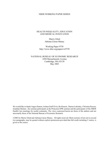
One obvious solution to this problem is to test the anomaly on an independent sample.Sometimes researchers use data from other countries, and sometimes they use data from priortime periods. If sufficient time elapses after the discovery of an anomaly, the analysis ofsubsequent data also provides a test of the anomaly. I supply some evidence below on the postpublication performance of several anomalies.The Size EffectBanz (1981) and Reinganum (1981) showed that small-capitalization firms on the NewYork Stock Exchange (NYSE) earned higher average returns than is predicted by the Sharpe(1964) – Lintner (1965) capital asset-pricing model (CAPM) from 1936-75. This “small-firmeffect” spawned many subsequent papers that extended and clarified the early papers. Forexample, a special issue of the Journal of Financial Economics contained several papers thatextended the size effect literature.2Interestingly, at least some members of the financial community picked up on the smallfirm effect, since the firm Dimensional Fund Advisors (DFA) began in 1981 with Eugene Famaas its Director of Research.3 Table 1 shows the abnormal performance of the DFA US 9-10Small Company Portfolio, which closely mimics the strategy described by Banz (1981).The measure of abnormal return αi in Table 1 is called Jensen’s (1968) alpha, from thefollowing familiar model:(Rit – Rft) αi βi (Rmt – Rft) εit,(1)where Rit is the return on the DFA fund in month t, Rft is the yield on a one-month Treasury bill,2Schwert (1983) discusses all of these papers in more detail.3Information about DFA comes from their web page: http://www.dfafunds.com and from the Center forResearch in Security Prices (CRSP) Mutual Fund database. Ken French maintains current data for the Fama-Frenchfactors on his web site: ench/.6
and Rmt is the return on the CRSP value-weighted market portfolio of NYSE, Amex, and Nasdaqstocks. The intercept αi in (1) measures the average difference between the monthly return to theDFA fund and the return predicted by the CAPM. The market risk of the DFA fund, measuredby βi, is insignificantly different from 1.0 in the period January 1982 – May 2002, as well as ineach of the three subperiods, 1982-1987, 1988-1993, and 1994-2002. The estimates of abnormalmonthly returns are between -0.2% and 0.4% per month, although none are reliably below zero.Thus, it seems that the small-firm anomaly has disappeared since the initial publication ofthe papers that discovered it. Alternatively, the differential risk premium for small-capitalizationstocks has been much smaller since 1982 than it was during the period 1926-1982.The Turn-of-the-Year EffectKeim (1983) and Reinganum (1983) showed that much of the abnormal return to smallfirms (measured relative to the CAPM) occurs during the first two weeks in January. Thisanomaly became known as the “turn-of-the-year effect.” Roll (1983) hypothesized that thehigher volatility of small-capitalization stocks caused more of them to experience substantialshort-term capital losses that investors might want to realize for income tax purposes before theend of the year. This selling pressure might reduce prices of small-cap stocks in December,leading to a rebound in early January as investors repurchase these stocks to reestablish theirinvestment positions.44There are many mechanisms that could mitigate the size of such an effect, including the choice of a tax year different from a calendaryear, the incentive to establish short-term losses before December, and the opportunities for other investors to earn higher returns byproviding liquidity in December.7
Table 1Size and Value Effects, January 1982 – May 2002Performance of DFA US 9-10 Small Company Portfolio relative to the CRSP value-weightedportfolio of NYSE, Amex, and Nasdaq stocks (Rm) and the one-month Treasury bill yield (Rf),January 1982 – May 2002. The intercept in this regression, αi, is known as “Jensen’s alpha”(1968) and it measures the average difference between the monthly return to the DFA fund andthe return predicted by the CAPM.(Rit – Rft) αi βi (Rmt – Rft) εitThe last row shows the performance of the DFA US 6-10 Value Portfolio from January 1994 –May 2002. Heteroskedasticity-consistent standard errors are used to compute the t-statistics.Sample Periodαiβit(αi 0)t(βi 1)DFA 9-10 Small Company 20020.00350.661.0130.150.816-2.14DFA US 6-10 Value Portfolio1994-2002-0.0022-0.598
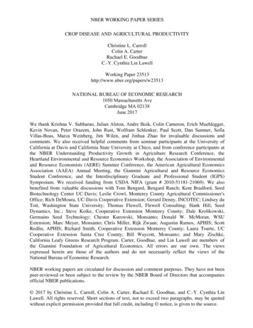
Table 2 shows estimates of the turn-of-the-year effect for the period 1962-2001, as wellas for the 1962-1979 period analyzed by Reinganum (1983), and the subsequent 1980-1989 and1990-2001 sample periods. The dependent variable is the difference in the daily return to theCRSP NYSE small-firm portfolio (decile 1) and the return to the CRSP NYSE large-firmportfolio (decile 10), (R1t - R10t). The independent variable, January, equals one when the dailyreturn occurs during the first 15 calendar days of January, and zero otherwise. Thus, thecoefficient αJ measures the difference between the average daily return during the first 15calendar days of January and the rest of the year. If small firms earn higher average returns thanlarge firms during the first half of January, αJ should be reliably positive.Unlike the results in Table 1, it does not seem that the turn-of-the-year anomaly hascompletely disappeared since it was originally documented. The estimates of the turn-of-theyear coefficient αJ are around 0.4% per day over the periods 1980-1989 and 1990-2001, which isabout half the size of the estimate over the 1962-1979 period of 0.8%. Thus, while the effect issmaller than observed by Keim (1983) and Reinganum (1983), it is still reliably positive.Interestingly, Booth and Keim (2000) have shown that the turn-of-the-year anomaly isnot reliably different from zero in the returns to the DFA 9-10 portfolio over the period 19821995. They conclude that the restrictions placed on the DFA fund (no stocks trading at less than 2 per share or with less than 10 million in equity capitalization, and no stocks whose IPO wasless than one year ago) explain the difference between the behavior of the CRSP small-firmportfolio and the DFA portfolio. Thus, it is the lowest-priced and least-liquid stocks thatapparently explain the turn-of-the-year anomaly.This raises the possibility that marketmicrostructure effects, especially the costs of illiquidity, play an important role in explainingsome anomalies (see Chapters 12 (Stoll) and 21 (Easley and O’Hara)).9
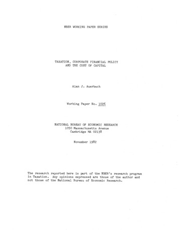
Table 2Small Firm/Turn-of-the-Year Effect, Daily Returns, 1962-2001(R1t - R10t) α0 αJ Januaryt εtR1t is the return to the CRSP NYSE small-firm portfolio (decile 1) and R10t is the return to theCRSP NYSE large-firm portfolio (decile 10). January 1 when the daily return occurs duringthe first 15 calendar days of January, and zero otherwise. The coefficient of January measuresthe difference in average return between small- and large-firm portfolios during the first twoweeks of the year versus other days in the year. Heteroskedasticity-consistent standard errors areused to compute the t-statistics.α0t(α0 0)αJt(αJ 990-2001-0.00026-1.720.005655.37Sample PeriodThe Weekend EffectFrench (1980) observed another calendar anomaly. He noted that the average return tothe Standard & Poor's (S&P) composite portfolio was reliably negative over weekends in theperiod 1953-1977. Table 3 shows estimates of the weekend effect from February 1885 to May2002, as well as for the 1953-1977 period analyzed by French (1980) and the 1885-1927, 19281952, and 1978-2002 sample periods not included in French’s study. The dependent variable isthe daily return to a broad portfolio of U.S. stocks. For the 1885-1927 period, the Schwert(1990) portfolio based on Dow Jones indexes is used. For 1928-2002, the S&P composite10
portfolio is used. The independent variable, Weekend, equals one when the daily return spans aweekend (e.g., Friday to Monday), and zero otherwise. Thus, the coefficient αW measures thedifference between the average daily return over weekends and the other days of the week. Ifweekend returns are reliably lower than returns on other days of the week, αW should be reliablynegative (and the sum of α0 αW should be reliably negative to confirm French’s (1980)results).The results for 1953-1977 replicate the results in French (1980). The estimate of theweekend effect for 1928-1952 is even more negative, as previously noted by Keim andStambaugh (1984). The estimate of the weekend effect from 1885-1927 is smaller, about halfthe size for 1953-1977 and about one-third the size for 1928-1952, but still reliably negative.Interestingly, the estimate of the weekend effect since 1978 is not reliably different from theother days of the week. While the point estimate of αW is negative from 1978-2002, it is aboutone-quarter as large as the estimate for 1953-1977, and it is not reliably less than zero. Theestimate of the average return over weekends is the sum α0 αW, which is essentially zero for1978-2002.Thus, like the size effect, the weekend effect seems to have disappeared, or at leastsubstantially attenuated, since it was first documented in 1980.The Value EffectAround the same time as early size effect papers, Basu (1977, 1983) noted that firms withhigh earnings-to-price (E/P) ratios earn positive abnormal returns relative to the CAPM. Manysubsequent papers have noted that positive abnormal returns seem to accrue to portfolios ofstocks with high dividend yields (D/P) or to stocks with high book-to-market (B/M) values.11
Table 3Day-of-the-Week Effects in the U.S. Stock Returns,February 1885 – May 2002Rt α0 αW Weekendt εtWeekend 1 when the return spans Sunday (e.g., Friday to Monday), and zero otherwise. Thecoefficient of Weekend measures the difference in average return over the weekend versus otherdays of the week. From 1885-1927, Dow Jones portfolios are used (see Schwert (1990)). From1928-May 2002, the Standard & Poor’s composite portfolio is used. Heteroskedasticityconsistent standard errors are used to compute the t-statistics.α0t(α0 005-1.37Sample PeriodαWt(αW 0)Ball (1978) made the important observation that such evidence was likely to indicate afault in the CAPM rather than market inefficiency, because the characteristics that would cause atrader following this strategy to add a firm to his or her portfolio would be stable over time andeasy to observe. In other words, turnover and transactions costs would be low and informationcollection costs would be low. If such a strategy earned reliable “abnormal” returns, it would beavailable to a large number of potential arbitrageurs at a very low cost.More recently, Fama and French (1992, 1993) have argued that size and value (asmeasured by the book-to-market value of common stock) represent two risk factors that are12
missing from the CAPM. In particular, they suggest using regressions of the form:(Rit – Rft) αi βi (Rmt – Rft) si SMBt hi HMLt εit(2)to measure abnormal performance, αi. In (2), SMB represents the difference between the returnsto portfolios of small- and large-capitalization firms, holding constant the B/M ratios for thesestocks, and HML represents the difference between the returns to portfolios of high and low B/Mratio firms, holding constant the capitalization for these stocks. Thus, the regression coefficientssi and hi represent exposures to size and value risk in much the same way that βi measures theexposure to market risk.Fama and French (1993) used their three-factor model to explore several of the anomaliesthat have been identified in earlier literature, where the test of abnormal returns is based onwhether αi 0 in (2). They found that abnormal returns from the three-factor model in (2) arenot reliably different from zero for portfolios of stocks sorted by: equity capitalization, B/Mratios, dividend yield, or earnings-to-price ratios. The largest deviations from their three-factormodel occur in the portfolio of low B/M (i.e., growth) stocks, where small-capitalization stockshave returns that are too low and large-capitalization stocks have returns that are too high (αi 0).Fama and French (1996) extended the use of their three-factor model to explain theanomalies studied by Lakonishok, Shleifer, and Vishny (1994). They found no estimates ofabnormal performance in (2) that are reliably different from zero based on variables such asB/M, E/P, cash flow over price (C/P), and the rank of past sales growth rates.In 1993, Dimensional Fund Advisors (DFA) began a mutual fund that focuses on smallfirms with high B/M ratios (the DFA US 6-10 Value Portfolio). Based on the results in Famaand French (1993), this portfolio would have earned significantly positive “abnormal” returns of13
about 0.5% per month over the period 1963-1991 relative to the CAPM. The estimate of theabnormal return to the DFA Value portfolio from 1994-2002 in the last row of Table 1 is -0.2%per month, with a t-statistic of -0.59. Thus, as with the DFA US 9-10 Small Company Portfolio,the apparent anomaly that motivated the fund’s creation seems to have disappeared, or at leastattenuated.Davis, Fama, and French (2000) collected and analyzed B/M data from 1929 through1963 to study a sample that does not overlap the data studied in Fama and French (1993). Theyfound that the apparent premium associated with value stocks is similar in the pre-1963 data tothe post-1963 evidence. They also found that the size effect is subsumed by the value effect inthe earlier sample period. Fama and French (1998) have shown that the value effect exists in asample covering 13 countries (including the U.S.) over the period 1975-1995. Thus, in samplesthat pre-date the publication of the original Fama and French (1993) paper, the evidence supportsthe existence of a value effect.Daniel and Titman (1997) have argued that size and M/B characteristics dominate theFama-French size and B/M risk factors in explaining the cross-sectional pattern of averagereturns. They conclude that size and M/B are not risk factors in an equilibrium pricing model.However, Davis, Fama, and French (2000) found that Daniel and Titman’s results do not hold upoutside their sample period.The Momentum EffectFama and French (1996) have also tested two versions of momentum strategies.DeBondt and Thaler (1985) found an anomaly whereby past losers (stocks with low returns inthe past three to five years) have higher average returns than past winners (stocks with highreturns in the past three to five years), which is a “contrarian” effect. On the other hand,14
Jegadeesh and Titman (1993) found that recent past winners (portfolios formed on the last yearof past returns) out-perform recent past losers, which is a “continuation” or “momentum” effect.Using their three-factor model in (2), Fama and French found no estimates of abnormalperformance that are reliably different from zero based on the long-term reversal strategy ofDeBondt and Thaler (1985), which they attribute to the similarity of past losers and smalldistressed firms. On the other hand, Fama and French are not able to explain the short-termmomentum effects found by Jegadeesh and Titman (1993) using their three-factor model. Theestimates of abnormal returns are strongly positive for short-term winners.Table 4 shows estimates of the momentum effect using both the CAPM benchmark in (1)and the Fama-French three-factor benchmark in (2).The measure of momentum is thedifference between the returns to portfolios of high and low prior return firms, UMD, whereprior returns are measured over months -2 to -13 relative to the month in question.5 The sampleperiods shown are the 1965-1989 period used by Jegadeesh and Titman (1993), the 1927-1964period that preceded their sample, the 1990-2001 period that occurred after their paper waspublished, and the overall 1927-2001 period. Compared with the CAPM benchmark in the toppanel of Table 4, the momentum effect seems quite large and reliable. The intercept α is about1% per month, with t-statistics between 2.7 and 7.0. In fact, the smallest estimate of abnormalreturns occurs in the 1965-1989 period used by Jegadeesh and Titman (1993) and the largestestimate occurs in the 1990-2001 sample after their paper was published.65This Fama-French momentum factor for the period 1927-2001 is available from Ken French’s web en.french/ftp/F-F Momentum Factor.zip.6Jegadeesh and Titman (2001) also show that the momentum effect remains large in the post 1989 period. Theytentatively conclude that momentum effects may be related to behavioral biases of investors.15
Table 4Momentum Effects, 1927 – 2001UMDt α β (Rmt – Rft) s SMBt h HMLt εtUMDt is the return to a portfolio that is long stocks with high returns and short stocks with low returns inrecent months (months -13 through -2). The market risk premium is measured as the difference in returnbetween the CRSP value-weighted portfolio of NYSE, Amex and Nasdaq stocks (Rm) and the one-monthTreasury bill yield (Rf). SMBt is the difference between the returns to portfolios of small- and largecapitalization firms, holding constant the B/M ratios for these stocks, and HMLt is the differencebetween the returns to portfolios of high and low B/M ratio firms, holding constant the capitalization forthese stocks. Heteroskedasticity-consistent standard errors are used to compute the t-statistics.SamplePeriodSampleSize, Tαt(α 0)βt(β 0)st(s 0)ht(h 0)Single-Factor CAPM 072.71-0.063-0.56Three-Factor Fama-French 01-1.830.0930.54-0.245-1.3516
Fama and French (1996) noted that their three-factor model does not explain themomentum effect, since the intercepts in the bottom panel of Table 4 are all reliably positive. Infact, the intercepts from the three-factor models are larger than from the single-factor CAPMmodel in the upper panel.Lewellen (2002) has presented evidence that portfolios of stocks sorted on size and B/Mcharacteristics have similar momentum effects as those seen by Jegadeesh and Titman (1993,2001) and Fama and French (1996).He argues that the existence of momentum in largediversified portfolios makes it unlikely that behavioral biases in information processing are likelyto explain the evidence on momentum.Brennan, Chordia, and Subrahmanyam (1998) found that size and B/M characteristics donot explain differences in average returns, given the Fama and French three-factor model. LikeFama and French (1996), they found that the Fama-French model does not explain themomentum effect. Finally, they found a negative relation between average returns and recentpast dollar trading volume. They argue that this reflects a relation between expected returns andliquidity as suggested by Amihud and Mendelson (1986) and Brennan and Subrahmanyam(1996).Thus, while many of the systematic differences in average returns across stocks can beexplained by the three-factor characterization of Fama and French (1993), momentum cannot.Interestingly, the average returns to index funds that were created to mimic the size and valuestrategies discussed above have not matched up to the historical estimates, as shown in Table 1.The evidence on the momentum effect seems to persist, but may reflect predictable variation inrisk premiums that are not yet understood.17
2.2Predictable Differences in Returns Through TimeIn the early years of the efficient markets literature, the random walk model, in whichreturns should not be autocorrelated, was often confused with the hypothesis of market efficiency(see, for example, Black (1971)). Fama (1970, 1976) made clear that the assumption of constantequilibrium expected returns over time is not a part of the efficient markets hypothesis, althoughthat assumption worked well as a rough approximation in many of the early efficient marketstests.Since then, many papers have documented a small degree of predictability in stockreturns based on prior information. Examples include Fama and Schwert (1977) [short-terminterest rates], Keim and Stambaugh (1986) [spreads between high-risk corporate bond yieldsand short-term interest rates], Campbell (1987) [spreads between long- and short-term interestrates], French, Schwert, and Stambaugh (1987) [stock volatility], Fama and French (1988)[dividend yields on aggregate stock portfolios], and Kothari and Shanken (1997) [book-tomarket ratios on aggregate stock portfolios]. Recently, Baker and Wurgler (2000) have shownthat the proportion of new securities issues that are equity issues is a negative predictor of futureequity returns over the period 1928-1997.An obvious question given evidence of the time-series predictability of returns is wheth
G. William Schwert Simon School of Business University of Rochester Rochester, NY 14627 and NBER Schwert@schwert.ssb.rochester.edu. 3 1 Introduction Anomalies are empirical results that seem to be inconsistent with maintained theories of asset-pricing behavior. They indicate either market inefficiency (profit opportunities) or