Transcription
TEMPERATURE INVESTIGATION IN REAL HOT RUNNER SYSTEM USING A TRUE3D NUMERICAL METHODTzu-Chau Chen1, Yan-Chen Chiu1, Marvin Wang1, Chao-Tsai Huang1, Cheng-Li Hsu2, Chen-YangLin2, Lung-Wen Kao21. CoreTech System (Moldex3D) Co., Ltd., ChuPei City, Hsinchu, Taiwan2. ANNTONG Co., Ltd., Sanchong, New Taipei City, TaiwanAbstractHot runner technology has been the solutions to themolding problems on many plastic injection products,such as automobile bumper, LCD/TV cover, bottle capand so on. However, the mechanism behind the hot runnersystem is too complicated to be fully understood. Inaddition, there exist some critical issues in the current hotrunner technology, such as temperture control issues, flowimbalance, and material degradation. As a result, thesimulation technolgy is highly needed for hot runnerdesigners and makers to examine their designs before thereal manufacturing. Through simulation analyses,designers and manufafctuers are able to catch the potentialissues on their hot runner systems and revise their designs.Hot runner simulation technology helps with theinvestigations into the behavior in hot runner system. Inthis paper, a true 3D numerical method is proposed andapplied to investigate the temperature behavior in a realhot runner system for PC material. The experiment isconducted and the simulating result is compared with thatfrom the experiment for the validation purpose.IntroductionRunner system plays a very important role ininjection molding process [1-4]. The purpose of runners isto transport melt from injection machine nozzle to thecavities. Runner designs have a great influence on thequalities of molded parts. The quality runner design isvery helpful in improving product qualities. However,traditional cold runner systems have certain inherentissues, such as material waste, regrind problem, increasedmolding cycle and so on. Moreover, poor productcosmetics, such as welding line and low gloss matter, arecommonly seen with the use of traditional cold runner. Asa result, hot runner technology [5-10] has become thetrend in order to deal with these issues in injectionmolding process. Hot runner technology can provide thebenefits of reduced injection pressure/clamping forcerequired, easy cavity filling, decreased cycle time,improved product quality, and energy/material saving. Forhot runner applications, it has been applied to many largesized plastic parts, such as bumper, automobile dashboard,TV/LCD front/back cover etc. Hot runner technology isalso used for some common plastic products: bottle caps,food plastic containers and so on.A hot runner system is mainly composed of hotrunner gate, , hot nozzle, manifold and heating coil. Thereare various types of desgins for each component. Forexample, hot runner gate options are very diverse,including hot-tip gate, thermal sprue gate, edge gate, andvalve gate. The combinations of different componentdesigns affect the hot runner system performance. Thedimension of each compoent is also very influential to itsbehavior. Hence, the mechanism in the hot runner systemis so complicated that it is difficult to be fully understood.In addition, there exist some critical issues in the currenthot runner technology, such as temperture control issues,flow imbalance, and material degradation. As a result, asimulation technolgy is highly required for hot runnerdesigners and makers to examine their designs before thereal prodcution. Through simulation analysis results,designers and manufafctuers are able to investigatetmperture profile, pressure drop, shear heating effect etc.and find the potential issues on their hot runner systems.Hot runner simulation technology is very useful inunderstaning complex hot runner system. Therefore, it canhelp improve hot runner system designs and productqualities.In this paper, a true 3D numerical method isproposed to simulate the behavior of a real hot runnersystem for PC material. The CAE model can beconstructed without too much effort by importing eachmajor hot runner components, defining their attributes,meshing automatically. The boundary conditions, heatconduction faces, can be also properly defined to matchwith the experiment. The dynamic melt temperatureprofile in the hot runner system can be simulated andinvestigated. The real hot runner experiment is conductedand the temperature is measured at the locations of interest.The simulating results are compared with those from theexperiment to validate this simulation technology. The
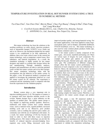
preliminary result indicates good agreement both in trendand magnitude.Numerical SimulationA true 3D numerical method is developed and usedto simulate the behavior of hot runner systems. The CAEmodel can be created without too much effort by usingMoldex3D. Each major hot runner component is imported,attribute-defined, and meshed automatically in thepreprocessing stage. Also, the boundary conditions can bedefined to match with the experiment in a convenient way.The defined BC surfaces are assumed direct contact withthe metal mold. The heat escapes from these areas due toheat conduction. On the other hand, the undefined surfacesare assumed contact with air. Those areas do not havecontributions to heat loss in the simulation analysis.Heating coils can be imported in .stl format to match withthe real geometry in the experiment. In the simulation,heating coils can be controlled by two heating methods: bytemperature or by power. For “by temperature”, theheating coils are given a specific temperature ( ) andmaintain this value all the time in the analysis. For “bypower” method, the heating coils are given a power value(W or W/cm 2) and controlled by “on/off” method. Eachheating coil is assigned a sensor node. This sensor nodedetects the temperature and determines whether thecorresponded heating coil is switched on or off. The targettemperature and range need to be defined for the analysis.A three-dimensional, cyclic, transient heatconduction problem with boundary conditions on hotrunner component surfaces is involved. The overall heattransfer phenomenon is governed by a three-dimensionalPoisson equation [11-15].Where n is the normal direction of mold boundary, h isheat transfer coefficient. On the exterior surfaces of themoldbase, (4)h hair , T0 Tair for r mDescription of CAE ModelIn this study, this numerical simulation technology isapplied to a real hot runner system manufactured byANNTONG IND. CO. LTD. This system includes thepart, hot runner nozzle, 3 sets of heating coils, 3 brassbushings which the heating coils are wrapped around, ametal mold, and other bushing components. Thedimension of the entire moldbase is 250.00 x 250.00 x320.00 mm. The material for the metal mold is P20. Thethermoplastic material for the melt is PC (Panlite L1225Y). The constructed CAE model for this hot runnersystem is shown in Figure 1. The figure 1 also indicatesthe materials used for each hot runner component. Thecomponent shown in the same color is made of the samematerial. 2T 2T 2T T(1) k 2 2 2 t y z xwhere T is the temperature, t is the time, x , y , and zare the Cartesian coordinates, is the density, Cp is thespecific heat, k is the is the thermal conductivity. The Cpequation holds for both hot runner components and partcomponent except with different thermal properties. Theinitial mold temperature is assumed to be equal to theinput of initial settings. The initial part temperaturedistribution is obtained from the analysis results at the endof filling and packing stages. Tc ,T 0, r Tp r , for r m for r p(2)In this study, the effect of thermal radiation is ignored.The conditions defined over the boundary surfaces andinterfaces of the mold are specified as,for t 0, km T h T To n(3)Fig. 1 The CAE model for hot runner systemTable 1 Material property for hot runner components
Table 1 lists the material properties, including density,heat capacity and thermal conductivity, for each hotrunner components in this system. These parameters arethe inputs in the analysis. This is to consider the effectsfrom different thermal properties.The figure 2 shows the information of boundaryconditions and sensor node locations which is definedaccording to the real experiments. The surfaceshighlighted in dark green color are defined as the contactareas with the metal mold. The undefined surfaces areautomatically assumed as heat insulation due to air layeraround these areas. The air is assumed as very poor heatconduction material. The number 1 to 10 sensor nodes areused to measure melt temperature function of time. Thesenodes are placed along the central line of hot runnernozzle. The number 11 to 17 sensor nodes (or 1A, 2A, 3A,1B, 2B, 3B, 1C) are used to control on/off for the heatingcoils. For example, the sensor nodes 12, 13, and 14 (or 1A,2A, 3A) are assigned to each heating coils respectively.The target temperature is 280 and the range is 2 .The power for each heating coil is 400W or 610W asindicated in figure 3. If the sensor node 1A reaches thetemperature of 282 , the corresponding heating coil isswitched off. On the contrary, if the temperature goesdown to 278 , the heating coil is turned on. This is thesame for the sensor nodes 2A, 2B and their correspondedheating coils.referred from the process condition in the real injectionmolding experiments. They are counted in one injectionmolding cycle for transient cool analysis. Therefore, thecycle time is 35 seconds. The melt temperature on thesensor nodes 1 to 10 can be predicted and compared withthe experimental measurements.Fig. 3 Heating coils and cooling channelExperimental StudyIn the hot runner experiment, the injection moldingprocess is conducted cycle by cycle. The melt temperatureis measured at the same locations as the positions ofsensor nodes 1 to 10 in the simulation. There are sevensensor lines arranged in the hot runner system which arerepresented by the sensor nodes (1A, 2A, 3A, 1B, 2B, 3B,1C) in the simulation. The figure 3 shows hot runnersystem used in the experiment. The heating coils areconnected to the power supplier. The figure 4 shows themetal mold in the experiment. The size of the moldbase is250.00 x 250.00 x 320.00 mm. The figure 5 shows sensorlines embedded in the grooves of the hot runner nozzle.Each line is 0.2mm in diameter. The lines are connected tothe power monitor for control of the heating coils. Table 2shows the molding parameters. The temperaturemeasuring will be applied after ten shots to make sure themelt temperature is stable.Fig. 2 Boundary conditions and sensor node positionsThe filling time and packing time are both 5seconds. The cooling channel layout and coolant (water)temperature is also shown in figure 3.The cooling timeand open time is 20s and 5s respectively. They areFig. 4 The hot runner system in the experiment
The Simulation ResultsThe figure 7 displays the simulating melttemperature field inside the runner or melt channel at theend of ten injection molding cycles. The sensor node 2detects higher melt temperature in the runner due to higherpower from the heating coil around that area. The sensornode 10 detects much lower melt temperature because ofthe cooling channel and heat conduction contact with themetal mold in the hot runner system. The melt temperaturefield at different timing can be shown and observed also.Fig. 5 Experimental metal moldFig. 6 Temperature sensor lines in the hot runner systemTable 2 Injection molding process parametersInjection molding process conditionFilling speed (mm/s)Injection time (s)Melt temperature ( )Mold temperature ( )Packing pressure (MPa)Packing time (s)Cooling time (s)Mold open time (s)Cycle time (s)4052808010520535Fig. 7 Temperature profile in the runner after ten injectionmolding cyclesThe figure 8 demonstrates the simulatingtemperature field inside of the moldbase after ten injectionmolding cycles. The moldbase near the cooling water haslower temperature as indicated in dark blue color.Results and DiscussionsThe simulating results are shown and discussed first,including melt temperature distribution inside of the meltchannel and moldbase. The dynamic temperature historycurves obtained from the sensor nodes are also displayedand investigated. In the experimental result, the melttemperature as function of the certain locations ismeasured and plotted. The simulating result is comparedwith that from the experiment. The comparison shows thegood agreement both in trend and magnitude. This is tovalidate this simulation technology used for hot runnersystem.Fig. 8 Temperature profile inside of moldbase after teninjection molding cycles
The figure 11 shows the experimental melttemperature distributions as function of location usingcontrolling sensor nodes 1C, 2A, and 3A. Both theexperimental and simulation results are similar to the caseof controlling sensor nodes 1A, 2A, and 3A.Fig. 9 Melt temperature history curves for t the sensornodes 1 to 10.The figure 9 displays the simulating melttemperature history curves for the sensor nodes 1 to 10.This records the dynamic response of melt temperaturecycle by cycle and allows for melt temperatureinvestigation at the end of the specific cycle by extractingthe data. It can be observed that the melt temperature ondetected from each sensor node goes up cycle after cycle.Ultimately, the temperature should reach steady state aftera long time. In this case, the temperature variation issmaller than 0.5% after ten molding cycles or 350 seconds.That means the melt temperature is nearly stable aftermany injection molding cycles.Fig. 11 Melt temperature distribution function of locationfor 1C, 2A, and 3A controlling sensor nodesThe figure 12 shows the experimental melttemperature distributions as function of location usingcontrolling sensor nodes 1B, 2B, and 3B. In theexperiment result, there is not obvious higher temperatureregion at the position of 60mm. The simulation result alsoindicates this phenomenon. This is different with theprevious two cases.The Validation from the ExperimentThe figure 10 shows the experimental melt temperaturedistributions as function of location using controllingsensor nodes 1A, 2A, and 3A. The position zero means thelocation of the gate. The temperature was measured afterseveral injection molding cycles and assumed to reachsteady state. The simulating result is also plotted togetherand compared with the experimental one.Fig. 12 Melt temperature distribution function of locationfor 1B, 2B, and 3B controlling sensor nodesIn the above three cases with different sets of controllingsensor nodes, the comparisons between the simulating andexperimental results indicate good agreement in both trendand magnitude.ConclusionsFig. 10 Melt temperature distribution function of locationfor 1A, 2A, and 3A controlling sensor nodesIn this research, a true 3D numerical method topredict the temperature behavior in the hot runner systemhas been developed. A hot runner system CAE model can
be constructed, attribute-defined, and meshed in anefficient way in the preprocessing step. Through thisnumerical technique, the dynamic feature of temperaturefield in hot runner systems can be simulated andinvestigated. A real case from ANNTONG hot runnersystems was used for the simulation. The simulating melttemperature profile can be obtained. The experimentalstudy for this hot runner system is conducted and the melttemperature is measured at the locations of interest. Thenumerical results are compared with those from theexperiment to validate Moldex3D simulation technologyapplied in this work. The simulating results are in goodagreement with those from the experimental in both trendand 14.15.T. A. Osswald, L Turng and P. J. Gramann, InjectionMolding Handbook, 2nd Ed., Hanser GardnerPublications, 2007.S. Y. Yang and L. Lien, Intern. Polymer Procession,XI, 2, p188, 1996.S. Y. Yang and L. Lien, Advances in PolymerTechnology, 15, 3, p205, 1996.S. C. Chen, Y. C. Chen and H. S. Peng, Journal ofApplied Polymer Science, 75, p1640, 2000.D. O. Kazmer, R. Nagery, B. Fan, V. Kudchakar, S.Johnston, ANTEC Tech. Papers 2005, 536.G. Balasubrahmanyan, David Kazmer, ANTEC Tech.Papers 2003, 387.Kapoor, D., Multi Cavity Melt Control in InjectionMolding, M. S. Thesis, Submitted to the Universityof Massachusetts, Amherst, December 1997.D. Frenkler, H. Zawistowski, “Hot Runners inInjection Moulds”, Rapra publishers, Shawbury 1998,p.267.B. Fan, D. Kazmer, ANTEC Tech. Papers 2003, 622.Peter Unger, “Hot Runner Technology”, HanserGardener Publication, 2006.S. C. Chen, Y. C. Chen and N. T. Cheng, Int. Comm.Heat Mass Transfer, 25, 7, p907, 1998.C. H. Wu and Y. L. Su, Int. Comm. Heat MassTransfer, 30, 2, p215, 2003.W. B. Young, Applied Mathematical Modelling, 29,p955, 2005.R. Y. Chang and W. H. Yang, Int. J. NumericalMethods Fluids, 37, p125, 2001.F. P. Incropera and D. P. DeWitt, “Introduction toHeat Transfer”, John Wiley & Sons Inc, 1996.Key Words: Hot runner; nozzle; heating coils;transient cool; Poisson’s equation
Hot runner technology has been the solutions to the molding problems on many plastic injection products, such as automobile bumper, LCD/TV cover, bottle cap and so on. However, the mechanism behind the hot runner system is too complicated to be fully understood. In addition, there exist some critical issues in the current hot .