WIXLIB

R. Abbate3. Decomposing the Cost of Credit and FundingMany market practitioners incorporate the market price of counterparty credit risk and one’s own credit risk into theirvaluation models. Some participants even incorporate the cost of funding into the prices quoted to commercial end-users.In the sections that follow, we examine the effects of credit risk and funding costs on the prices of financial derivativecontracts.3.1. The Counterparty’s Credit RiskAlthough research on counterparty credit risk (CCR) began in the 1990s, market participants became keenly aware of itsimportance as the global financial crisis of 2007-2008 unfolded. Regulations such as the Dodd-Frank Act and the ThirdBasel Accord (Basel III), along with fair-value accounting rules such as Accounting Standards Codification (ASC)Topic 820 and International Financial Reporting Standards (IFRS) 13, require credit risk to be reflected in the fair valuemeasurement of financial derivative contracts. In order to accurately price a derivative contract, one must include thecredit risk associated with one’s counterparty.Historically, banks have defaulted very rarely and commercial end-users have defaulted only occasionally. In December 2009, the Basel Committee on Banking Supervision (BCBS) concluded that approximately one-third of thelosses during the financial crisis can be attributed to actual counterparty default. The remaining two-thirds of the lossesresulted from the negative impacts of credit market volatility on banks’ earnings (Bank for International Settlements,2009). The BCBS consultative document indicated that “ the current framework addresses CCR as a default and credit mitigation risk, but does not fully account for market value losses short of default” (Bank for International Settlements, 2009). In response to this shortcoming, the BCBS introduced a new capital charge in Basel III: the Credit Valuation Adjustment (CVA).CVA is the present value of the expected loss on a trade or portfolio of trades due to default by one’s counterparty.Stated differently, CVA is a price that represents the difference in value between a default-free value of a counterparty’sportfolio and the value of the same portfolio taking into account the possibility of the counterparty’s default. CVAmeasures the sensitivity of a trade’s exposure to movements in a counterparty’s credit spread - not counterparty default,per se.The approaches to calculate CVA range from relatively simple “add-on” methods to complex Monte Carlo simulation.The chosen method depends principally on the sophistication and various resources available to the market participant. Tocompute CVA, banks commonly rely on Monte Carlo simulation, which becomes computationally intensive as the sizeof the portfolio and the number of simulated risk factors (e.g. interest rates, foreign exchange rates, commodity prices,etc.) increase. The reader is referred to Appendix A of this paper for the general process by which CVA would be computed under a Monte Carlo simulation approach.Prior to the onset of the financial crisis, banks typically viewed themselves as default-free, while viewing their corporate end-user clients as subject to default. If both parties were to agree to this framework, and assuming that there isno collateral posted 4, as is often the case with transactions occurring with commercial end-users (Watt, 2011), then wehave what is referred to as Unilateral CVA (UCVA). UCVA is the risk-neutral expectation of the discounted loss and canbe expressed from the bank’s perspective as𝑇𝑇𝑈𝑈𝑈𝑈𝑈𝑈𝑈𝑈 𝐿𝐿𝐿𝐿𝐿𝐿 𝑃𝑃(𝑡𝑡) 𝐸𝐸𝐸𝐸(𝑡𝑡) 𝑑𝑑𝑃𝑃𝑃𝑃𝐶𝐶 (0, 𝑡𝑡)(3.1)0where 𝐿𝐿𝐿𝐿𝐿𝐿 (Loss Given Default) equals one minus the recovery rate 5, 𝑃𝑃(𝑡𝑡) is the discount factor process for time 𝑡𝑡,𝐸𝐸𝐸𝐸(𝑡𝑡)is the risk-neutral expectation of the exposure to a given counterparty at time 𝑡𝑡 and 𝑑𝑑𝑃𝑃𝑃𝑃𝐶𝐶 (0, 𝑡𝑡) is the counterparty’s default probability distribution. These default probabilities can be derived by bootstrapping the counterparty’scredit default swap (CDS) spreads or reasonable proxies thereof, taking into account the counterparty’s geographic region,industrial sector and rating (sometimes referred to as “mark-to-matrix”). We note in Equation (3.1) that the exposure is4On September 3, 2014, the Board of Governors of the Federal Reserve system and other federal ‘prudential regulators’ re-proposed rules that wouldexempt non-financial “commercial” end-users from posting margin on non-cleared derivatives. On September 17, 2014, the CFTC re-proposed rulesthat are largely identical to those re-proposed by the prudential regulators.5Typically 35% to 40% for non-distressed entities.59

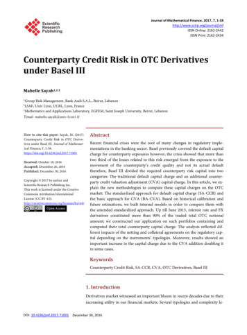
R. Abbateindependent of counterparty default (i.e. there is no “wrong-way” risk 6) and that the exposures are obtained usingrisk-neutral probabilities.In order to compute the UCVA of a fixed/floating swap, for example, we simulate 𝑗𝑗 number of relevant risk factorsusing 𝑛𝑛 number of random variables across 𝑖𝑖 number of time steps. Credit exposure can be viewed as a function ofthe risk factors that drive the values of the derivative contracts in the portfolio. Let us assume that a given risk factor 𝑆𝑆follows a geometric Brownian motion with drift 𝜇𝜇 and volatility 𝜎𝜎. Let us further assume an initial value of zero, a localdrift of 2% and a diffusion of 25%. Figure 1 depicts the evolution of risk factor 𝑆𝑆 based on fifty 7 simulated paths 8across 120 time steps. The simulated values of risk factor 𝑆𝑆 greater than zero represent an expected positive exposure forthe payer of the swap at each point in time.The Expected Exposure (EE) is the mean of the distribution of positive exposures at any particular future date prior tothe maturity of the longest-dated transaction in the netting set 9. The EE at time 𝑡𝑡 can be written as𝑁𝑁𝐸𝐸𝐸𝐸(𝑡𝑡) 𝔼𝔼 𝑚𝑚𝑚𝑚𝑚𝑚 𝑖𝑖 1𝑉𝑉𝑖𝑖 (𝑡𝑡), 0 (3.2)exposurewhere 𝔼𝔼 denotes the expectation operator, 𝑁𝑁 denotes the number of transactions in the netting set and 𝑉𝑉𝑖𝑖 (𝑡𝑡) denotesthe value of the 𝑖𝑖-th trade at time 𝑡𝑡. Figure 2 depicts the Expected Exposure based on the simulations in Figure 1.86420-2-4-6-801224364860728496 108 120monthexposureFigure 1. Simulated Exposure; μ 2%, σ 25%. Source: 0-0.50012243648607284EEEEEENE96 108 120yearFigure 2. Expected Exposure, Effective Expected Exposure, Expected Negative Exposure. Source: Author.6Occurs when exposure to a particular counterparty is adversely correlated with the credit quality of that counterparty.For illustration purposes; in practice, we set 𝑛𝑛 5000.8We use a Marsenne Twister pseudo-random number generator to create standard normal random variables.9A group of transactions with a single counterparty that are subject to a legally enforceable bilateral netting agreement.760

R. AbbateThe Effective Expected Exposure (EEE) at a specific date, as depicted in Figure 2, is the maximum Expected Exposure occurring at that date or any prior date (i.e. constrained to be non-decreasing) and is expressed as𝐸𝐸𝐸𝐸𝐸𝐸(𝑡𝑡𝐸𝐸 ) 𝑚𝑚𝑚𝑚𝑚𝑚𝑡𝑡 [0,𝑡𝑡 𝐸𝐸 ] 𝐸𝐸𝐸𝐸(𝑡𝑡) (3.3)We apply the EE from the simulations in Figure 1, the term structure of U.S. dollar discount factors (as of September19, 2014) depicted in Figure 3 and the hypothetical CDS spreads depicted in Figure 4 to Equation (3.1). When assuming a recovery rate of 40%, the CVA amounts to 0.04064. We depict the CVA in Figure 5. Appendix B contains a tableof results for counterparty default probability, EE and CVA.The tenor of the trade and the creditworthiness of one’s counterparty are the two primary drivers of CVA. Long-datedtrades tend to be the most CVA-intensive. In general, the presence of a master netting agreement, collateral arrangementsand termination provisions tend to reduce the exposure, and thus the UCVA.We can extend Equation (3.1) and express CVA more formally as𝑇𝑇 𝐶𝐶𝐶𝐶𝐶𝐶 (1 𝑅𝑅𝑐𝑐 )𝔼𝔼𝑡𝑡 𝜆𝜆𝑐𝑐 (𝑢𝑢) 𝑣𝑣𝑡𝑡 (𝑢𝑢) 𝐶𝐶(𝑢𝑢) 𝑃𝑃𝐸𝐸 (𝑡𝑡, 𝑢𝑢) 𝑑𝑑𝑑𝑑 𝑡𝑡discount 496 108 120monthbasis pointsFigure 3. Term structure of U.S. dollar discount factors. Source: Author.180160140120100806040200CDS ( counterparty )CDS ( self )1224364860728496108 120monthFigure 4. Term structure of CDS spreads. Source: Author.61(3.4)

R. 0.020%-0.030%-0.040%CVADVA01224364860728496 108 120monthFigure 5. Credit Valuation Adjustment, Debit Valuation Adjustment. Source: Author.where 𝑅𝑅𝑐𝑐 denotes the recovery rate applied to one’s counterparty, 𝜆𝜆𝑐𝑐 denotes the survival probability (hazard rate)applied to one’s counterparty, 𝑣𝑣𝑡𝑡 denotes the future value of the derivative contract, 𝐶𝐶 denotes the value of the collateral and 𝑃𝑃 denotes the discount factor 10. In Equation (3.4), we are concerned with the uncollateralized positive exposure.Basel III mandates the calculation of a CVA capital charge, the purpose of which is to improve banks’ ability to withstand potential mark-to-market losses associated with deterioration in the creditworthiness of their counterparties tonon-cleared derivative contracts. Banks also seek to optimize the use of regulatory capital by determining the marginalimpact of trades on risk weighted assets and regulatory capital. At this time, most of the large global banks have incorporated CVA into the prices of derivatives contracts they quote to clients. These banks commonly recover the cost ofthe CVA by pricing it upfront. The quotes from offshore banks may differ from those of local banks in that the offshorebanks may include a sovereign credit risk premium in the CVA calculation.The CVA calculation depends on the entire portfolio of transactions. Thus, it is not possible to assign amark-to-market value to a particular transaction without consideration of the other transactions in the portfolio. Additionally, CVA involves significant model risk. According to Brigo et al. (2013), “ five banks might compute CVA in15 different ways”.Basel III mandates that banks can use two different methods to calculate CVA. The advanced approach requires theuse of Monte Carlo simulation, wrong-way risk, stress testing, back testing and stressed effective expected positive exposure (EEPE) 11. This approach, which applies to most of the largest banks, results in lower capital requirements. To theextent that a particular bank has regulatory approval to use the Internal Model Method (IMM) for calculating counterparty credit risk capital, then the advanced approach must be used. Otherwise, banks are required to use the standardizedapproach, which allows for two methods. The Current Exposure Method (CEM), which allows banks to apply relativelycrude add-ons to the mark-to-market value of transactions, has been widely criticized for its significant shortcomings,most notably understating the benefit of netting and collateral. The Standardized Method (SM), which relies on a formulaic approach, is more risk-sensitive than the CEM. The new standardized approach (SA-CCR), which replaces CEMand SM and is intended to better recognize the effects of netting and collateral, becomes effective on January 1, 2017.The management of CVA varies considerably across organizations. Some banks calculate CVA only for the purposesof accounting/reporting and regulatory capital. Others banks have implemented a CVA pricing framework, under whichCVA is incorporated into the inception price of client trades. Because a counterparty’s CDS spreads can exhibit highvolatility (particularly during times of market stress), some banks have established centralized CVA desks, which consolidate and centrally manage the enterprise-wide CVA. These CVA desks have a mandate that ranges from passivelyhedging the P&L associated with CVA volatility to actively managing CVA by trading specific reference entities inorder to allow the bank to transact additional business with a client whose credit line would otherwise prevent such10Typically a blended interest rate that takes into account the interest rate of the collateral and the funding rate.EEPE is the weighted average of the expected exposure.1162

R. Abbatetrading. Banks may enter into single-name credit default swaps, single-name contingent credit default swaps (CCDS) orother equivalent hedging instruments which reference the entity directly. The lack of liquidity in the CDS market andthe unavailability of single-name CDS are often cited as challenges to hedging CVA volatility.In the case of a 5-year uncollateralized trade with a commercial end-user, the increase in required capital could besignificant. In view of higher capital charges, some banks have reevaluated the economics of their OTC trading businesses. Meanwhile, many smaller banks have not implemented a CVA pricing framework, allowing them to quote morecompetitive prices than the larger global banks and to compete for client business that would not have been possiblebefore the large global banks implemented their CVA pricing frameworks. Until smaller regional banks implement aCVA pricing framework, large global banks are left striking a delicate balance between prudent pricing and the need towin trades with end-user clients.Legislators in the European Union have provided European banks an exemption from calculating a CVA capitalcharge for corporates, sovereigns and pension funds. Banks in the U.S. are justifiably concerned that the absence of asimilar exemption in the U.S. rules gives an unfair pricing advantage to banks trading within the European Union,which are not required to hold capital against similar exposures. Other critics have argued that the CVA exemption isinconsistent with aims to achieve globally harmonized prudential requirements.Intermezzo: Potential Future ExposureCounterparty exposure is the larger of zero and the market value of a transaction or portfolio of transactions within anetting set that would be lost if a given counterparty were to default and there were zero recovery during a bankruptcyproceeding. Current Exposure (CE) is the current mark-to-market exposure to a given counterparty and is also referredto as the replacement cost. CE is not particularly useful as a credit risk metric, since it is a single point estimate and failsto provide a robust indication of credit risk at future points in time.Potential Future Exposure (PFE), also referred to as Peak Exposure (PE), is a high percentile (e.g. 95%) of thedistribution of exposures at any particular future date prior to the maturity of the longest-dated transaction in the nettingset. PFE is typically computed with simulation models (e.g. Monte Carlo simulation). For each future date 𝑡𝑡, the valueof a transaction or portfolio of transactions with a given counterparty is simulated.The curve PE(t) is the peak exposure profile up to the final maturity of the portfolio. If we denote the confidenceinterval as α, then the peak exposure for a future scenario at time 𝑡𝑡 is written as𝑃𝑃𝑃𝑃(𝑡𝑡) 𝑖𝑖𝑖𝑖𝑖𝑖{𝑋𝑋(𝑡𝑡): 𝑃𝑃[𝑃𝑃𝑃𝑃𝑃𝑃(𝑡𝑡) 𝑋𝑋(𝑡𝑡)] 1 𝛼𝛼}(3.5)For example, PFE generated with 95% statistical confidence represents the level of potential exposure that is exceeded with only 5% probability.Netting agreements function to mitigate credit risk among counterparties. Under the terms of a netting agreement,transactions in the netting set with negative mark-to-market values are used to offset transactions with positivemark-to-market transactions; only the net positive mark-to-market value represents the credit exposure at the time ofdefault. In the absence of a netting agreement, and assuming no recovery, we can express PFE as𝑁𝑁𝑃𝑃𝑃𝑃𝑃𝑃Π (𝑡𝑡) 𝑖𝑖 1𝑚𝑚𝑚𝑚𝑚𝑚(𝑉𝑉𝑖𝑖 (𝑡𝑡), 0)(3.6)where Π denotes the portfolio of transactions, 𝑁𝑁 denotes the number of transactions in the portfolio and 𝑉𝑉𝑖𝑖 (𝑡𝑡) denotes the value of the 𝑖𝑖-th trade at time 𝑡𝑡.In the presence of a netting agreement, we can express PFE as𝑁𝑁𝑃𝑃𝑃𝑃𝑃𝑃Π (𝑡𝑡) 𝑚𝑚𝑚𝑚𝑚𝑚 𝑖𝑖 1𝑉𝑉𝑖𝑖 (𝑡𝑡), 0 (3.7)The maximum value of PFE(𝑡𝑡) over any given time horizon is referred to as the Maximum Potential Future Ex63

R. Abbateexposureposure (MPFE), as depicted in Figure 6.PFE is analogous to Value-at-Risk (VaR), with a few exceptions. VaR represents exposure due to market losses (i.e.left tail of the distribution), while PFE represents exposure due to market gains (i.e. right tail of the distribution). Whereas VaR typically addresses a short time horizon, PFE looks many months or years into the future. Lastly, PFErepresents a distribution of outcomes, rather than a single point estimate.A counterparty’s credit exposure profile can be segmented into a “diffusion phase” and an “amortization phase”.During the diffusion phase, the passage of time increases the probability that the underlying risk factors drift significantly from their initial values. During the diffusion phase of the exposure profile, a trade has a long time to maturity,many remaining cash flows and is sensitive to market uncertainty. The diffusion is determined primarily by the volatility of the underlying risk factors. During the amortization phase, the passage of time results in a reduction in the numberof cash flows that would need to be replaced in the event of default. During the amortization phase of the exposure profile, a trade has a short time to maturity, few remaining cash flows and has little sensitivity to market uncertainty. Theoffsetting nature of the diffusion phase and the amortization phase creates the humped-back appearance in a counterparty’s exposure profile (assuming contracts do not have a final exchange of notional), as depicted in Figure 6. Fortrades with multiple cash flows, the PFE typically peaks at a point in time that is approximately one-third to one-halfinto the life of the 200.00PFEMPFE01224364860728496 108 120monthFigure 6. Potential Future Exposure at 95% confidence. Source: Author.3.2. One’s Own Credit RiskPrior to the onset of the financial crisis, many banks relied on UCVA to manage counterparty credit risk. This approachis justified when one of the two parties to the transaction can be considered default-free, as many banks were prior toAugust 2007. In the aftermath of the financial crisis, however, we know that banks are susceptible to default.Let us assume that two parties use UCVA to value a particular transaction. One party is a highly rated credit; the other party is not. The parties will likely arrive at different valuations for the same trade due to the differing assumptions ofcounterparty risk (e.g. probability of default) that each party assigns to the other. This asymmetry is addressed by incorporating Debit Valuation Adjustment 12 (DVA). Unlike CVA, DVA represents the difference in value between adefault-free portfolio and the value of the same portfolio that incorporates the possibility of the one’s own default.The inclusion of DVA has been widely debated and remains controversial. Companies record gains when their owncreditworthiness deteriorates, and record losses when their own creditworthiness improves. When a firm’s credit spreadswiden, DVA increases, reflecting a reduction in the value of its liabilities resulting from the increased probability ofdefault. For example, in Q1 2009, Citibank reported a positive mark-to-market due to a worsening of its credit quality,citing that “Revenues also included a net 2.5 billion positive CVA on derivative positions, excluding monolines,mainly due to the widening of Citi’s CDS spreads” (Citibank, 2009). In October 2011, the Wall Street Journal reportedthat Goldman Sachs’ “DVA gains in the third quarter totaled 450 million, about 300 million of which was recordedunder its fixed-income, currency and commodities trading segment ” (Brigo et al., 2013).12Also referred to as Debt Valuation Adjustment.64

R. AbbateThere is an offsetting effect between CVA and DVA. If one party records a CVA loss, the other party records a corresponding DVA gain. The inclusion of DVA results in a Bilateral Valuation Adjustment (BVA), which is also referredto as Bilateral CVA (BCVA).Notwithstanding the controversy, ASC 820 (formerly Statement of Financial Accounting Standards 157) defines fairvalue as “the price that would be received to sell an asset or paid to transfer a liability in an orderly transaction betweenmarket participants at the measurement date”. Fair-value accounting standards require the inclusion of DVA in derivatives prices. ASC 820 “ clarifies that a fair value measurement for a liability reflects its nonperformance risk (the riskthat the obligation will not be fulfilled). Because nonperformance risk includes the reporting entity’s credit risk, the reporting entity should consider the effect of its credit risk (credit standing) on the fair value of the liability in all periodsin which the liability is measured at fair value under other accounting pronouncements ” (Financial Accounting Standards Board, 2011). Despite the relevant accounting standards, Basel III no longer permits the offsetting of CVA withDVA.We can express DVA as𝑇𝑇 𝐷𝐷𝐷𝐷𝐷𝐷 (1 𝑅𝑅𝑠𝑠 )𝔼𝔼𝑡𝑡 𝜆𝜆𝑠𝑠 (𝑢𝑢) 𝑣𝑣𝑡𝑡 (𝑢𝑢) 𝐶𝐶(𝑢𝑢) 𝑃𝑃𝐸𝐸 (𝑡𝑡, 𝑢𝑢) 𝑑𝑑𝑑𝑑 𝑡𝑡(3.8)where 𝑅𝑅𝑠𝑠 denotes the recovery rate applied to one’s self, 𝜆𝜆𝑠𝑠 denotes the survival probability (hazard rate) applied toone’s self, 𝑣𝑣𝑡𝑡 denotes the future value of the derivative contract, 𝐶𝐶 denotes the value of the collateral and 𝑃𝑃 denotesthe discount factor. In Equation (3.8), which follows from Equation (3.4), we are concerned with the negative uncollateralized exposure. Figure 2 depicts Expected Negative Exposure (ENE), which is the mean of the distribution of negative exposures at any particular future date prior to the maturity of the longest-dated transaction in the netting set. Theequation for ENE is identical to Equation (3.2), except that we replace the 𝑚𝑚𝑚𝑚𝑚𝑚 function with the 𝑚𝑚𝑚𝑚𝑚𝑚 function.We apply the ENE from the simulations in Figure 1, the term structure of U.S. dollar discount factors (as of September 19, 2014) depicted in Figure 3 and the hypothetical CDS spreads depicted in Figure 4 to Equation (3.8). When assuming a recovery rate of 40%, the DVA amounts to 0.02765. We depict the DVA in Figure 5. Appendix B contains atable of results for default probability, ENE and DVA.Apart from its counterintuitive nature, another criticism of DVA is the difficulty one faces when attempting to hedgeit or monetize it. Some argue that DVA is not merely an accounting adjustment, but instead can be monetized throughreplication strategies. Hedging DVA involves buying one’s own bonds or, for example, selling a credit default swap ona basket of one’s closely correlated peers (since a bank cannot sell credit default swaps on itself) 13. Burgard and Kjaer(2010) derive a partial differ

contracts to account for the effects of counterparty credit risk, one's own credit risk and the cost of funding. We discuss the impact of Credit Valuation Adjustment (CVA), Debit Valuation Adjustment (DVA) and Funding Valuation Adjust-ment (FVA), collectively referred to as xVA, on the price of a derivative contract. 2.