Transcription
2170IEEE TRANSACTIONS ON WIRELESS COMMUNICATIONS, VOL. 7, NO. 6, JUNE 2008A Software-Defined Radio System forBackscatter Sensor NetworksGiovanni Vannucci, Senior Member, IEEE, Aggelos Bletsas, Member, IEEE, and Darren Leigh, Member, IEEEAbstract—Backscatter radio is proposed for sensor networks.In that way, the transmitter for each sensor is simplified toa transistor connected to an antenna and therefore, the costfor each sensor’s communicator becomes negligible, while energy used for wireless communication per sensor is minimized.A software-defined transceiver is built to transmit a carrier,receive the reflections from various sensors and extract theirtransmitted messages. This work presents a thorough modelof the backscatter radio link, the system architecture and aset of data extraction techniques for each sensor’s information,testing in practice a sensor communicating through backscatterat a range of approximately 15 meters indoors, with 5 milliwatttransmission power at 10 bits per second. This work highlightsthe idiosyncrasies of the backscatter channel and provides a newcommunication perspective in the fertile area of scalable sensornetworks, especially when low bit-rate, ultra-low cost sensors arerequired.Index Terms—RFID, fading channel, bit error rate, wirelesssensor networks.I. I NTRODUCTIONTHE technique of radio backscatter is commonly usedin RFID (Radio Frequency IDentification) systems. Ina typical application, a RFID tag communicates to a reader(sometimes called an interrogator) its identification numberand in some cases additional information stored in its memory.Radio backscatter communication is an attractive solutionin such systems because the tag does not need to activelytransmit any radio signal; the tag simply reflects a radio signaltransmitted by the interrogator and modulates the reflection,by controlling its own reflection coefficient [1]–[3]. This leadsto very-low-cost implementations and also very low powerrequirements in the tag. Indeed, in systems where the distancebetween tag and interrogator is short (i.e., less than 2-5 m orso), RFID tags may derive their power from the signal receivedfrom the interrogator. Such batteryless tags are known as“passive” and the maximum distance (range) achieved by suchsystems is determined by the tag’s ability to extract enoughvoltage from the received signal. Even though passive RFIDtechnology has matured since the first work on modulatedbackscattered signals [1], the range of typical passive RFIDsystems is limited, at most within a room [4], spanning aManuscript received October 6, 2006; revised July 11, 2007; acceptedSeptember 4, 2007. The Associate Editor coordinating the review of thispaper and approving it for publication was A. Stefanov. This researchwas supported by Mitsubishi Electric Research Laboratories (MERL), 201Broadway Avenue, Cambridge, MA 02139 USA. Part of this work waspresented at IEEE PIMRC 2007, Athens Greece.The authors are with Mitsubishi Electric Research Laboratories (MERL),201 Broadway Avenue, Cambridge, MA 02139 USA (e-mail: {vannucci,leigh}@merl.com, aggelos@media.mit.edu).Digital Object Identifier 10.1109/TWC.2008.060796.variety of applications from classical supply chain monitoringand inventory control to non-traditional applications such asmusic interfaces [5].By contrast, RFID systems that require a larger operating distance use tags that are known as “semi-passive” (or“battery-assisted” [6]). Such tags include a battery but, liketheir passive counterparts, they too use backscatter (ratherthan active transmission) as the communication mechanism(e.g. [7]). The battery is used only to operate the tag statemachine and the backscatter modulator and, as a result, it ispossible for such tags to communicate over longer ranges. Themaximum range of a semi-passive tag depends on the signalto-noise ratio (SNR) available at the interrogator receiver. Thisin turn, depends on system parameters such as the powerlevel transmitted by the interrogator, the reflection efficiencyof the tag, the SNR efficiency of the modulation scheme, thenoise figure of the interrogator receiver, the radio-propagationenvironment, as well as the bit-rate.In many RFID implementations, bit rates have to be relatively high because the RFID tag needs to convey its messageto the interrogator in a fraction of a second (eg. [8]). Bycontrast, in sensor networks this limitation does not usuallyapply. In this work, an architecture for a wireless sensor network is presented, based on radio backscatter communicationwhere the operating range can be as large as 100 metersoutdoors. The long range is made possible, in part, by the useof extremely low bit rates between the “tags” (the sensors, inthis case) and the “interrogator” (referred to as hub, in thiscase). Even bit rates as low as 10 bps or less are acceptablebecause the sensors are at fixed locations, continuously ableto backscatter the signal from the hub. In many applications,the sensors need to transmit observed data (e.g. temperature)at intervals of seconds to minutes. Thus, a continuous bit-rateof just a few Hz is adequate in applications where relatively“slow” environmental changes are monitored.Utilizing backscatter for sensor networks provides a lowcomplexity and ultra low-cost solution for each sensor transmitter, since the latter could consist of a single RF transistorswitch. Apart from the attractive simplicity of the sensortransmitter, backscatter radio simplifies the overall networkarchitecture, since all sensors (tags) unidirectionally transmittowards the interrogator (hub), as opposed to more involvednetwork architectures that rely on multi-hop, self-organized(ad hoc) routing. In [9], a comparison of energy consumptionbetween active RFID (single-hop) and typical wireless sensornetwork (multi-hop) is attempted, revealing relevant dependencies of communication range and sensor topology on theoverall energy budget. In [10], the performance of an ALOHAc 2008 IEEE1536-1276/08 25.00
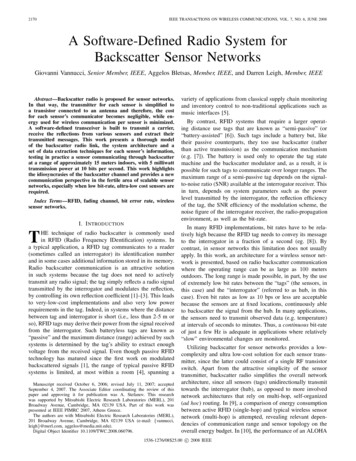
VANNUCCI et al.: A SOFTWARE-DEFINED RADIO SYSTEM FOR BACKSCATTER SENSOR NETWORKS2171access scheme is modeled and analyzed for an active RFIDsystem where tags only transmit short bursts of their uniqueidentification number.Despite its attractive conceptual simplicity, backscatter radiofor sensor networks as envisioned in this work, must take intoaccount unique constraints (idiosyncracies):i. Ultra-low complexity sensors: Sensors (tags) in this workmeet very stringent requirements of low cost, low powerand small size. The transmitter of each sensor consistsof a single transistor that switches antenna impedancebetween two states, while coding and signal conditioningare extremely simple. However, the hub receiver includesmore sophisticated signal processing to offset, as muchas possible, this limitation.ii. Unidirectional communication: In many typical RFIDapplications, tags include a receiver. This allows the tagto detect when it interferes (collides) with other tags andsimplifies multiple-access by allowing the interrogator tocontrol tag transmissions. That is the key idea behindAloha-based or tree-based anti-collision algorithms [11].By contrast, sensors in this work do not have a receiverand thus, there is no mechanism for coordination orsynchronization among them [12]. As such, anti-collisionalgorithms found in the RFID literature are not an option.iii. Continuous sensor operation: All sensors in this workcontinuously backscatter their information. As such, thepresented system contrasts with prior systems designedto acquire information from a subset of tags (or a singletag) within a fraction of time and not continuously (seefor example pioneering RFID work in [8]).iv. Ultra-fast varying multi-path: Multi-path is not considered a major problem in typical RFID systems becauseradio propagation is usually “line of sight” (LOS) andthe bit rate is sufficiently high that, if multi-path occurs,it affects received signal strength in an approximatelyconstant fashion over the duration of the message. Bycontrast, the much lower bit-rate in this work means thatphase and amplitude of the received signal may changesubstantially due to multi-path, over time intervals as shortas a couple of bits, even for static (not mobile) sensors.This work provides a detection scheme that is tolerant ofsuch impairments.Consequently, the contributions of this paper are summarized below:a. A thorough model of the backscatter wireless channel thathighlights its distinctive characteristics and serves as a solidframework for future research in relevant problems such aschannel access, signal processing and detection techniquesfor backscatter radio sensor networks.b. A concrete set of signal and data extraction techniquesfor each sensor’s information, especially suited to theunidirectional character and fast varying multi-path natureof backscatter channel, as well as the continuous operationof all sensors.c. A proof-of-concept demonstration of backscatter communication for ultra low-cost sensor networks with a completehardware and flexible software prototype, using a desktoppersonal computer (PC).SensorsHubFig. 1. Layout of a Backscatter-based sensor network. Several low-costsensors modulate and reflect a carrier transmitted by a central station (hub).Tx AntRF OscillatorSplitterRF CarrierreferenceRx AntPower AmplifierICPUADCHomodyneQ RF front endControlRF ImpedanceswitchSensorPCHubFig. 2. Backscatter communication between the hub and a single sensor.Notice that the transmitting element at the sensor, is simply a switch madeof a transistor.The presentation is divided in two parts: Section II describesthe system architecture, including the basic assumptions andsystem equations, modulation and access scheme used by allsensors, as well as a summary of the radio prototype. SectionIII describes data extraction for each sensor, including alltechniques used for signal filtering, detection and synchronization. Techniques are evaluated with simulation as wellas experimental results from the radio prototype. Finally,conclusion is provided in section IV.II. S YSTEM A RCHITECTUREA system of approximately N 100 200 ultra low-costsensors, located outdoors within approximately dmax 100meters from a central hub, is envisioned (Fig. 1). The sensorsmonitor and continuously report to the hub, one or moreenvironmental quantities that vary slowly with time. Therefore,the required bit-rate per sensor is limited, on the order of10 bps/sensor. Such slowly-varying environmental quantitiesinclude (but are not limited to) environmental pollutant concentration, humidity or temperature.A. The Radio LinkThe unmodulated radio-frequency (RF) carrier transmittedby the hub can be written asshub (t) 2PT exp j(ωc t φc ) ,(1)where PT , ωc , φc are the power, angular frequency and phaserespectively of the RF carrier transmitted from the hub.At distance di between hub and sensor i, the signal powerhas experienced “one-way” propagation link loss Li . It isassumed that the hub antenna is mounted at height hT and
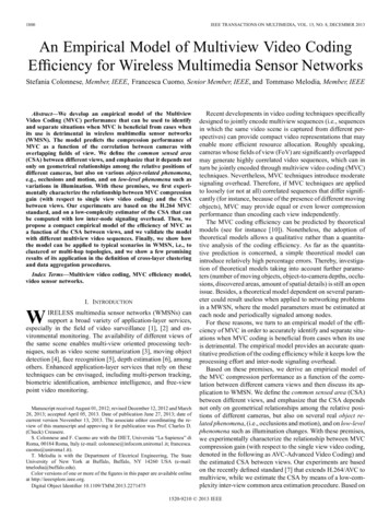
2172IEEE TRANSACTIONS ON WIRELESS COMMUNICATIONS, VOL. 7, NO. 6, JUNE 2008the sensor antenna at height hR . Taking into account the lineof-sight (LOS) path between hub and sensor antenna, as wellas one reflection from the ground, one-way loss Li can beapproximated by [13]: received powerGT GR (λ/4πdi )2 , if di d0 2 Li transmitted powerGT GR hT hR /di 2 , if di d0(2)where GT and GR are the gains of the transmitting (hub) andreceiving (sensor) antenna respectively, λ is the RF carrierwavelength and d0 is given by:4πhT hR.(3)λNotice that accounting for a single ground reflection, results tothe well-studied phenomenon of signal received power beingdecreased faster than in free space. In this simple scenario,received power drops between the second or fourth power ofdistance.At the sensor, the received signal ri (t) is simply reflectedback out of the same antenna that received it. Sensor information is modulated onto the reflected signal by varyingthe sensor’s reflection coefficient ηi (t). Sensor i accomplishesthis by controlling a semiconductor device (e.g. a field-effecttransistor (FET) or a diode) attached to the antenna (Fig. 2).Accordingly, the reflected signal can be written as:d0 si (t) ηi (t) ri (t).(4)In practical implementations of backscatter, the reflectioncoefficient has only two distinct possible states, and backscatter modulation is accomplished by alternating between thesetwo states. Because of that, the reflection coefficient can bewritten in terms of a binary function of time, bi (t), that onlytakes the values 1:ηi (t) η0 ηm bi (t),(5)where η0 represents a fixed (unmodulated) complex reflectionand ηm is the amplitude of the modulated component ofthe reflection. With this notation, the two possible complexreflection coefficients are η0 ηm and η0 ηm . The fixedreflection component adds a multitude of fixed reflectionsfrom all static scatterers in the environment and as such,it does not contribute in sensor backscatter communication.Consecutively, η0 is ignored and the above equation is simplywritten as:ηi (t) ηm bi (t).(6)Finally, the backscattered signal travels from sensor i back tothe hub and as such, experiences again power loss Li . Thelatter assumes that the hub receive antenna has the same gainand polarization as the hub transmit antenna. Thus, the powerof the received signal at the hub, due to backscatter operationat sensor i, is given from:Pihub PT L2i η,(7)where η is the reflection efficiency of the tag with valuedependent on ηm .1 For convenience, it is assumed that all1Adetailed analysis of optimization parameters related to reflection can befound in [14].Spectrum of Backscattered SignalCarrier FrequencyRF reflections dueto environmentN SubcarrierFrequencies forN SensorsModulated RFfrom a single sensor.fc -fsNfc -fs1fcfc f s1fc f sNBFig. 3. Spectrum of received signal at the hub receive (Rx) antenna, underthe basic assumptions of this work.sensors are made of the same materials and antenna designsand thus, reflection efficiency η, as well as ηm , are the sameacross all sensors. Consecutively, the backscattered signalreceived at the hub due to sensor i, can be written as a complexfunction of time:i(t) Ai (t) bi (t) exp(jωc t φ0 (t)),rhub(8)where Ai (t) is the (real) time-varying amplitude and φ0 (t) isthe time-varying carrier phase of the received signal, due tobackscatter operation of sensor i. Notice that both amplitudeand carrier phase are functions of time, given the time-varyingnature of the wireless channel between hub and sensor i.A thorough presentation regarding the time-varying natureof multi-path propagation in wireless channels is beyond thescope of this paper. For our purposes, it is sufficient to notethat carrier phase φ0 is time-varying and unknown, in general.B. The Modulation at Each SensorIn each sensor i, the function bi (t) generated by the controller is a square wave at a predetermined frequency, referredto as the subcarrier frequency fsi (or angular subcarrierfrequency ωsi ) of that sensor. Information from each sensoris modulated onto its unique subcarrier, i.e. different sensorshave different subcarrier frequencies. The available sensorsubcarrier frequency band is denoted as (fsMIN , fsMAX), withavailable bandwidth B fsMAX fsMIN (Fig. 3).Given that for sensor i, the subcarrier waveform bi (t) canonly take two values ( 1) in the implemented sensors, binarymodulation is the only option. Minimum shift keying (MSK)was chosen, which is a special case of frequency shift keying(FSK), because it has better power spectrum properties compared to other digital modulation techniques such as amplitudeshift keying or phase shift keying. Specifically, MSK has apower spectrum SMSK (f ) that drops as the fourth power offrequency [15]:SMSK (f ) 1,(5T f )4(9)
VANNUCCI et al.: A SOFTWARE-DEFINED RADIO SYSTEM FOR BACKSCATTER SENSOR NETWORKSas opposed to BPSK, where power spectrum drops as thesecond power of frequency [15]:SBPSK (f ) 1,(2πT f )2(10)where T is the symbol (bit) duration. This is a useful propertywhen two different sensors operate in closely adjacent subcarrier frequencies. In that case, utilization of MSK is preferableover BPSK (or ASK) simply because interference from onesensor to the other is minimized.2Consecutively, bi (t) is written as a square wave of angularfrequency ωsi , with angle modulation represented by φsi (t),in terms of its Fourier components:bi (t) 4 1cos (2k 1) ωsi t φsi (t) .π2k 1(11)k 0With FSK modulation and no baseband filtering (due to thesimple backscattering operation of each sensor), φsi (t) can bewritten as:t φsi (t) 2πΔfsBi [k] p(τ kT ) dτ,(12)0kwhere T is the bit duration, Bi [k] 1 is the information bitpattern of sensor i, p(t) is a rectangular pulse of duration Tand amplitude 1 and finally, Δfs is the frequency deviation.For MSK specifically, Δfs 0.25/T [15].The use of rectangular pulses (according to eq. (12) andΔfs 0.25/T ) simplified practical implementation of MSKmodulation at each sensor. Nevertheless, rectangular pulsesalso imply the existence of odd harmonics. In order to avoidinterference of third (or higher) harmonics of one sensor subcarrier to other sensor signals, the minimum sensor subcarrierfrequency utilized, should be chosen appropriately:fsMAX.(13)3The sensors and receiver built adhere to the above rule, withfsMAX 200 kHz and fsMIN 67 kHz.3 fsMIN fsMAX fsMIN C. The Hub Receiver RF Front-EndThe RF front-end of the hub receiver implemented in thiswork, only sees the fundamental component of the squarewave bi (t). This is done in order to simplify hub receiverdesign, as capturing higher harmonics would need a muchwider bandwidth than B fsMAX fsMIN . From (11), it canbe seen that the fundamental component holds 80% of thetotal power of the square wave. Therefore, including all theharmonics would, at best, improve signal strength by about 1dB. This does not justify the substantial additional cost andcomplexity associated with the wider bandwidth.Substituting the fundamental term from (11) into (8), thefollowing expression for the backscatter signal from sensor iis obtained: 4i(t) Ai (t) exp (jωc t φ0 (t)) cos ωsi t φsi (t) .rhubπ(14)2 Sensor subcarrier frequency allocation and relevant issues are discussedin detail in the subsection II-D.2173It is common in backscatter communication to use homodyne detection in the receiver. This is particularly effectivebecause the receiver is co-located with the source of the RFcarrier and, by using the transmitted signal itself as a reference for homodyne detection, phase noise cancels out ([16],pp. 129-138). For the purposes of this document, it is sufficientto note that a homodyne receiver removes the RF carrier (i.e.,the signal is frequency-shifted to 0-Hz center frequency) andextracts the real and imaginary part of the received signal (alsoreferred to as the “in-phase” and “quadrature” components).Thus, the output of the RF homodyne front-end is a pair ofreal signals for sensor i: yIi (t) (4/π) Ai (t) cos φ0 (t) cos ωsi t φsi (t) ,yQi (t) (4/π) Ai (t) sin φ0 (t) cos ωsi t φsi (t)(15)where yIi (t) is the real part of (14) (the “in-phase” component)and yQi (t) is the imaginary part of (14) (the “quadrature”component).Finally, taking into account backscattered signals from Nsensors, as well as noise at the receiver, the aggregate signalseen from the analog-to-digital converter (ADC) immediatelyafter the heterodyne front-end (Fig. 2), becomes:rI (t) N yIi (t) nI (t), rQ (t) i 1N yQi (t) nQ (t), (16)i 1where nI (t), nQ (t) represent additive receiver noise. Sourcesof receiver noise include thermal and quantization noise andthe two noise components above are assumed to be lowpass, independent and identically distributed Gaussian randomprocesses. The power spectral density of the noise is assumedflat, up to a cutoff frequency W , which denotes the homodyneRF front-end bandwidth. Their variance σ 2 is related to powerspectral density N0 by:σ 2 E n2I E n2Q W N0 .(17)The implemented homodyne RF front-end of this workhas bandwidth W 220 kHz, accommodating the selectedmaximum subcarrier frequency fsMAX 200 kHz and thus,the whole sensor subcarrier frequency range.D. The Sensors AccessEach sensor bit rate of R 1/T 10 bps is ordersof magnitude smaller than each sensor subcarrier frequencyfsi B [67 kHz, 200 kHz]. Therefore, eqs. (15) imply thateach sensor’s signal is a narrow-band signal centered aroundits own and unique subcarrier frequency, allowing multiplesensors to operate simultaneously in this subcarrier frequencyrange. Fig. 3 provides a snapshot of the received backscatteredsignal spectrum,3 around the carrier frequency fc . Notice thatRF clutter around the carrier frequency is typical, due toscatterers around the hub, and that is why fsMIN 0 Hz.The continuous operation of all sensors differentiates thiswork from traditional RFID systems, where usually the interrogator access a subset of the tags (sensors) within a3 This is the received signal at the hub receiver (Rx) antenna, beforeheterodyne downconversion to dc.
IEEE TRANSACTIONS ON WIRELESS COMMUNICATIONS, VOL. 7, NO. 6, JUNE 2008TABLE IS IMULATION PARAMETERS FOR E DGE C OLLISION P ROBABILITYE VALUATIONRdmaxdminPTfcGTGRhThRηN010 bps100 m10 m30 dBm900 MHz9 dB3 dB3m0.25 m-10 dB-164 dBm/Hz15Random Sensor Subcarrier Freqs (300 Sensors)Edge Collision (Outage) Probability (%)2174Random Sensor Subcarrier Freqs (100 Sensors)Equally Spaced Subcarrier Freqs (300 Sensors)12.5300 Sensors - Random Assignment of Subcarrier Freqs.107.55100 Sensors - Random Assignment of Subcarrier Freqs.2.5percentage of time (not continuously). The latter scenariooccurs when a) a single tag passes within working range ofthe interrogator [8], as in toll collection scenarios or b) tagsare equipped with receivers and can be addressed individually[17], or in groups with the help of a tree-based anti-collisionalgorithm (e.g. see [11]). The sensor access scheme in thiswork is, in principle, based on the limited required bandwidthfor each sensor and the fact that different sensors operate indifferent subcarrier frequencies, in conjunction with a flexibledata processor (discussed subsequently).In practice, given that sensors continuously modulate without any baseband filtering mechanism (due to backscatteroperation), adjacent in subcarrier frequency sensors mightinterfere with each other. This event might occur dependingon how close in subcarrier frequency are the sensors and howmuch different is their signal power. Following the notation ofthis work and particularly eqs. (7), (9), signal-to-interferenceand-noise ratio (SINR) can be calculated, as well as theprobability of SINR to fall below a target ratio (TR) forEb /N0 , required for successful reception: Pihub /RPr TR ,NN0 j i,j 1 SMSK ( fsj fsi ) Pjhub /R(18)where Eb denotes energy-per-bit. Notice that interference fromone sensor to another does not depend on the wireless environment between them, but instead, depends on the wirelessenvironment (and distance) between each sensor and the hub.This is another distinctive characteristic of backscatter radiodue to its two-way (from hub to sensor and back to hub),round-trip nature.Fig. 4 plots the above probability of outage (or sensorcollision, as commonly referred to in the RFID literature),for the worst-case scenario of sensor i located at the edge ofcoverage di dmax 100 meters. The rest of the sensors areuniformly distributed with ranges between 10 100 meters andsubcarrier frequencies randomly (i.e. not carefully) assigned.The list of parameters used are summarized in Table I. It isshown that for a moderate target ratio (TR) Eb /N0 of 6 dB,the worst-case collision event occurs with probability of 2.5% for 100 sensors or 8.5% for 300 sensors, when sensorsubcarrier frequencies are randomly assigned. We note thatthis is worst case scenario values, as a sensor located closerto the hub (and not at the edge of coverage), has strongerbackscattered signal. Still, these numbers indicate that a rather300 Sensors - Equal Spacing of Subcarrier Freqs.0012345678910Target Eb/N0 (dB)Fig. 4. Collision (outage) probability for a sensor located at the edge ofcoverage (100 m).limited number of sensors will not work (collide). This can becompensated by installing additional sensors into the network,given their reduced complexity and cost.The same plot shows that when subcarrier frequencies areequally spaced in the available range B, the above probabilitygoes to zero, even for 300 sensors. Between the two abovescenarios (random assignment or equally spaced subcarrierfrequencies), there is the alternative scenario of carefully allocating frequencies for sensors closer to the hub and randomlyassigning subcarrier frequencies for all the rest.Accordingly, sensor interference is not an issue for themajority of sensors in this system, under the aforementionedassumptions. The basic reason is the limited bandwidth neededfor each sensor, which is 3 4 orders of magnitude smallerthan the available subcarrier frequency band B, allowingsimultaneous operation of multiple sensors. A similar resultwas also reported in [18].Thereinafter, we strictly focus on sensors that do not collideand as such, any reference to noise will be limited to receivernoise. From eq. (15), the average energy per bit can be derived:Eb (16/π 2 ) A2i T /2,(19)and the SNR for sensor i information signal becomes:ρ Eb8 A2 T 2 2i .N0π σ /W(20)The formula above assumes coherent (optimal) combiningof the in-phase and quadrature components in eq. (15), as wellas stable signal amplitude Ai (t).4E. System Prototype Details1) Hub: The frequency of the transmitted RF carrier istunable in the range 900-930 MHz, with transmitted power at5 mW. A portion of the signal transmitted by the antenna isalso used as the local oscillator (LO) for homodyne receptionand down-conversion. As already mentioned, the bandwidthof the implemented RF front-end is W 220 kHz.4Ai (t) Ai constant, otherwise ρ becomes a function of time.
VANNUCCI et al.: A SOFTWARE-DEFINED RADIO SYSTEM FOR BACKSCATTER SENSOR NETWORKS2175Rx AntfrontendIQHomodyneRF front-end(a) Hub(b) SensorFig. 5. The hub includes a transmit (Tx) and a receive (Rx) antenna. Eachsensor built in this work consists of a bow-tie antenna connected to a transistor,controlled by a low-cost micro-controller and a large, manual switch (fordemonstration purposes).The result of the down-conversion is a pair of in-phase (I)and quadrature (Q) baseband waveforms, digitized by a dualchannel 16-bit analog-to-digital converter (ADC) (StrategicTest, Ultra-Fast series). The sampling rate is 1 MHz for eachwaveform (Figs. 2, 6). With this sampling rate, the Nyquistfrequency is 500 kHz which allows subcarrier frequencies upto fsMAX 200 kHz to be accurately recorded with enoughmargin for digital filtering of adjacent signals. The 16-bitresolution allows adequate dynamic range to accommodatesensors at various distances from the hub. The ADC boardis installed in a desktop personal computer (PC) and dataprocessing is performed completely in software. From thatperspective, the system described in this work is softwaredefined. Fig. 5(a) is a photo of the hub transmit and receiveantennas. The metal box between them provides a simple, yetefficient, separation between transmit and receive RF signals.2) Sensors: Each sensor is designed around a low-powermicro-controller (Texas Instruments MSP430) driving a lowpower RF switch. The micro-controller clock is derived from alow-cost watch-type crystal at 32768 Hz, with an accuracy of100 ppm. The specific subcarrier frequency for each sensor, inthe aforementioned range B [67 kHz, 200 kHz], is producedby a software-based phase-locked-loop (PLL), which makesFSK or MSK modulation easy to implement.Each sensor is battery-assisted and operates semi-actively:battery is only used for switching on/off a single transistor, performing subcarrier modulation, without any furthersignal conditioning, amplification or processing. Decouplingthe power requirements of each sensor to function from thepower required for successful communication allows backscatter radio operation in extended ranges. Furthermore, batteriesin sensors are commonly already available to power theelectronics required for monitoring a specific parameter ofinterest (eg. pollutant concentration, humidity etc). Fig. 5(b)is a photo of one of the sensors built for experimentation,where each sensor’s bow-tie antenna can be seen. Bow-tieantennas are easy to tune in a wide spectrum range aroundfc 900 MHz.Processingfor Tag 1ADCFFTPCProcessingfor Tag 2Processingfor Tag NFig. 6.The hub receiver architecture. In-phase (I) and quadrature (Q)component of the aggregate received signal is sampled and converted tothe frequency domain. Processing for each individual sensor follows usinga general purpose desktop computer.III. DATA P ROCESSINGData processing involves the software-defined part of thereceiver, which consists of a dual-channel ADC and a desktopPC. The received signal after homodyne RF processing (eq.(16)) is sampled and processed in software, with the followinggoals:1) to extract the useful narrow-band signals, around thesubcarrier frequencies of all sensors,2) to reduce the sampling rate appropriately, from 1 MHzto a few tens of Hz, given that memory and processingtime per sensor signal are practically limited, especiallywhen a large number of sensors is utilized, and3) to detect the transmitted bit patterns and synchronize tothe information bits for each sensor.The following subsections describe in detail the techniques(and their rationale) followed in this work.A. Sensor Signal AcquisitionThe first required task is to identify how many sensorsare operating and which are their respective subcarrier frequencies. Therefore, the average power spectrum is
2170 IEEE TRANSACTIONS ON WIRELESS COMMUNICATIONS, VOL. 7, NO. 6, JUNE 2008 A Software-Defined Radio System for Backscatter Sensor Networks Giovanni Vannucci, Senior Member, IEEE, Aggelos Bletsas, Member, IEEE, and Darren Leigh, Member, IEEE Abstract—Backscatter radio is proposed for sensor networks. In that way, the transmitter for each sensor is simplified to