Transcription
Predicting the Success of a Retirement PlanBased on Early Performance of InvestmentsCS229 Autumn 2010 Final ProjectDarrell Cain, AJ MinichAbstractIdeally, the retiree would like to select a rate thatresults in the funds being nearly completely exhaustedat the end of his or her life. (For the purposes of thispaper, we will assume that the retirement span r isexactly 30 years.) By setting the final amount Fr tozero, we can calculate a special IWR called the SafeWithdrawal Rate, or SWdR. The SWdR representsthe maximum amount a retiree can spend on a yearlybasis without borrowing – that is, the optimal balancebetween retirement lifestyle and financial security.This concept raises perhaps the most importantquestion in retirement: how does one decide his or herown SWdR? After all, the equation for IWR (and thusSWdR) depends on growth and inflation ratesthroughout the retirement, which the retiree obviouslydoes not know at the beginning of retirement. There isalso the issue that, historically, the variance can be quitelarge: the SWdR reaches as high as 15% in ‘good’ times(such as 1950-1980) and as low as 4% in depressedeconomies. Selecting a low SWdR hedges risk, but hasa significantly negative impact on the ‘golden years’ thatthe retiree has worked so hard to earn.The current approach was pioneered in 1994 byBengen1, and involves calculating the historical SWdRsfor an asset and then choosing the minimum of thosevalues. The approach relies on the idea that the marketwill perform no worse than it has at some point in thepast. For years, financial planners have used Bengen’smethod to attain the ‘Rule of 4%’, which (as mentionedabove) is the absolute minimum of all SWdRs in theperiod over which financial data is available (19262010).Although this approach promises 100%certainty of a successful retirement, it is ratherconservative, requiring the retiree to live as if theirretirement will span the worst economy in the lastcentury. Thus in the vast majority of cases, the Rule of4% leaves the retiree with significant savings at the endof retirement (experimentally, this can be as much as 14Using historical data on the stock market, it ispossible to predict the historical success rates of givenretirement plans. The fundamental problem withretirement planning is the inability to collect data on theperformance of the investments in the future. Thus aretiree often does not know whether or not his planwill succeed or fail until they are well into the planitself. In this paper, we address the effectiveness ofassessing a retirement plan based on the first few yearsof market performance.IntroductionMany wage-earners face great uncertainty uponentering retirement: even with enormous savings, theirown futures and the future of investment markets isimpossible to predict. Given the wide number ofvariables affecting their portfolio’s performance,retirement planning is often a long-term bet based onvery little information. A retiree’s worst financialnightmare, of course, is running out of savings beforehis end of life, so the consequences are dire if he placesthe wrong.To capture the predicament facing retirees, wedevelop an equation called the initial withdrawal rate(IWR) equation which gives the percentage amount ofthe initial savings that can be spent over each year(taking inflation into account). This equation predictsthe annual yearly buying power of a retiree over thecourse of their retirement:where gi is the growth of the assets in period i, infi theinflation in period i, r the number of retirement years,Fr the amount of money left over at the end ofretirement, and I0 the initial savings. (See Appendix:Calculating SWdR for a complete derivation.)1 William P. Bengen, Determining Withdrawal Rates Using HistoricalData, Journal of Financial Planning, October 1994, pp. 14–24.1
Predicting the Success of a Retirement Plan Based on Early Performance of Investmentstimes the initial portfolio value). As an added difficulty,the retiree will often adjust the yearly withdrawal ratebased on previous years’ rates, which increases theretirement-plan SWdR but adds nonlinear terms to theIWR equation. Bengen’s method cannot account erating suboptimal numbers even when the retireeperforms the most basic withdrawal adjustments.Though the retiree can increase his withdrawal rateabove Bengen’s conservative estimate during theretirement, he will need to live frugally in the early yearsof retirement and only increase his withdrawal rate nearthe end of the plan. This situation, too, is suboptimal:the retiree would prefer to live above his means duringthe first few years of retirement and make adjustmentsafter a certain number of years.We aim to develop and test an algorithm wherebya retiree could predict his retirement plan’s full-lengthSWdR after only five years of retirement. If it ispossible to predict the SWdR for a given retirementbefore the retirement is complete, then the retiree canadjust his income within a few years of enteringretirement. For the purposes of this paper, we willconsider the algorithm successful if, with only five yearsof retirement portfolio financial history, it predicts the30-year SWdR within 20% of the true value with 90%confidence.The output results are the actual Safe WithdrawalRates for the 30-year periods corresponding to the datasets. Thus we letSWdR for 30 year period in yeari.Given all input features , one can calculate theexact SWdRusing the equations discussed above.However, we focus on attaining sufficiently accurateSWdR when we limit the features down to only the firstyears of growth and inflation data. Thus wedefineThuswould be a set of input featurescontaining 5 years of growth/inflation data, and basedon a retirement portfolio beginning in year 6 of ourhistorical data (which is 1932, given that our databegins in 1926).Modeling with Linear RegressionFirst, we assume that the data follows a fairly linearrelationship, allowing us to use linear regression togenerate a model of the data. We select a value,define X to be a matrix containing successiveoneach row, and Y as a vector containing the values forthose corresponding years. In creating our linearregression model, we are looking for a hypothesisvector that satisfies(we have included a yintercept in our definition of). Thus as long as thetraining set contains more thanexamples, wecan solve our model using least-squares approximation:Creating a DatasetWe start by building a dataset on which to test ouralgorithms. We define the set of input features to bethe following parameters: Growth data g of each asset for each year of theretirement Inflation data inf for each year of the retirement Average return r of the entire portfolio for the 30year period Standard deviation σ of the portfolio for the 30year periodWe add the last two features primarily to differentiatebetween different portfolios which may have the sametypes of assets, but differing amounts of each.Thus for an n-year retirement period beginning inyear i, we define our vector of input features asFor each value of, we used atraining set composed of 100 different portfoliosbeginning in different years to generate our model, andthen ran our prediction on a test set containing k 10,000 such different portfolios. We define the error, mean errorand the failure rateasfollows:2
Error Relative to true SWdRPredicting the Success of a Retirement Plan Based on Early Performance of Investmentsperformance when more than seven years of data areavailable.However, when we investigate the size of themaximum errors affecting both the mean error and thefailure rate, we see that the model can generate trulyuseless results.In 10% of all instances, linearregression may predict a SWdR twice as much as theactual value, or it may predict that the retiree’s SWdR isnegative – he must continue adding money to fund his‘retirement’. While useful for giving us a baseline forperformance, linear regression fails to providesufficiently precise answers.Mean Error - Linear Regression16%14%12%10%8%6%4%2%0%1 3 5 7 9 11 13 15 17 19 21 23 25 27 29Number of Included Years (m)% of test instances with 20% relative error40%Modeling with a Support VectorMachineFailure Rate - Linear Regression35%Linear regression fails in part because it expectsthe values to lie along a hyperplane, despite theinherent nonlinearity of our problem.A moresophisticated fitting algorithm, such as a support vectormachine (SVM), could model these relationships andpredict SWdR values in a high-dimensional featurespace. Additionally, an SVM fits naturally with ourintuition that only certain growth and inflation rates inour input feature set – particularly the high-gain andhigh-loss years – will have a discernible impact on theactual SWdR value, and will thus become our supportvectors.Since an SVM mainly works as a binary classifier,we will modify the problem statement as follows: agiven withdrawal rate can be either above or below theSWdR, indicating the potential success or failure as aretirement plan. In this case, the SWdR serves as aboundary value between the set of all successful andfailure withdrawal rates. We choose a set of evenlyspaced withdrawal rates above and below the SWdR,and include these as input features along with thecorresponding growth and inflation rates. For eachwithdrawal rate below the SWdR, the classifier is 1(indicating a successful withdrawal rate), and for eachrate above the SWdR, it is -1 (indicating failure). Aftertraining the model and running a prediction, we identifythe original SWdR by feeding in several withdrawalrates along with the growth and inflation conditionsand identifying where the boundary lies.It is important to note that, while this methodresults in a better model, its error depends not only onthe classification success but also the spacingbetween the withdrawal rates used to create the new30%25%20%15%10%5%0%1Max Error Relativeto true SWdR140%2 3 4 5 6 7 8 9 10Number of Included Years (m)Max Error - Linear Regression120%100%80%60%40%20%0%1 3 5 7 9 11131517192123252729Number of Included Years (m)The figures above show the average error, thefailure rate and the maximum error across m. We cansee that the mean error reflects generally goodperformance, with relative accuracy dropping to within10% of the true value after onlyyears. Thefailure rate also reveals reasonable performance, withfewer than 10% of instances resulting in poor3
Mean Error - SVM10%8%6%4%2%0%1 3 5 7 9 11 13 15 17 19 21 23 25 27 29Number of Included Years (m)% of test instances with 20% relative error120%100%80%60%40%20%1Linear RegressionSVM30%Linear RegressionSVM0%Failure Rates Comparison35%Max Error Comparison140%Max Error Relative to true SWdRError Relative to true SWdRPredicting the Success of a Retirement Plan Based on Early Performance of Investments2 3 4 5 6 7 8 9 10Number of Included Years (m)satisfy our requirements: with, the cases offailure drops below 10%. Thus with the SVM, we havesuccessfully predicted SWdR within the desiredtolerance given only the first five years of retirementportfolio performance.Similarly, the maximum error with the SVM is wellbelow that of linear regression, especially forwhen it drops below 40% worst-case. This errorbound represents a significant improvement over linearregression, and proves that we may be confident in theresults generated using the SVM.25%20%15%10%5%0%1Conclusion2 3 4 5 6 7 8 9 10Number of Included Years (m)Although linear regression failed to provide asuccessful prediction algorithm, a standard SVM with alinear kernel met our criteria. With the SVM, we canpredict SWdR to within 20% in 90% of test cases, andto within 40% in all of the test cases. Although weimagine that a retiree would want better accuracy forthe purposes of retirement planning, we point out thatthe retiree must take on some risk in order to maximizethe annual withdrawal rate. Using our proposedmethod and taking on minimal risk, the retiree may (insome cases) withdraw 50% more from his portfolioannually than when using Bengen’s approach tocalculating the SWdR. With those additional funds, theretiree can enjoy more of the retirement funds he hasworked so hard during his life to earn.feature set. Even when the SVM properly classifies theboundary value, the resulting SWdR prediction can beas much as. Thus we will define the SVM's errornot as the ratio of misclassified training examples, butas the error between the predicted boundary value andthe actual SWdR. To minimize this value, we willdeclare a very small step size (typically around .0001,or .01%).The results for the described SVM 2 are shownabove. The method achieves excellent mean error,falling below 6% after 5 years. The failure rate results,compared above to those of linear regression, also2R.-E. Fan, K.-W. Chang, C.-J. Hsieh, X.-R. Wang, and C.-J. Lin.LIBLINEAR: A Library for Large Linear Classification, Journal ofMachine Learning Research 9 (2008), 1871-1874. Software available athttp://www.csie.ntu.edu.tw/ cjlin/liblinear.4
Predicting the Success of a Retirement Plan Based on Early Performance of InvestmentsAppendix: Calculating SWdROriginally written by Darrell Cain for Cain Watters and Associates.Utilizes historical financial data from IBB to calculate appropriateSWdR, given an initial portfolio and the years across which theretirement lasts.We now have the equation in a state where the CWR forthe initial amount can be explicitly solved. For a retirementover period r, the following equation holds.At the start of retirement an individual has an initialamount of savings. At any given point in time the individualwill withdraw a specific amount of money from that savings.For all analysis done the point of withdrawal is chosento be the end of the year. From this the current withdrawal rate(CWR) is defined.It is important that in each retirement scenario thetheoretical retiree does not use information from future years.This is important because this is the case in actual retirement.Therefore withdrawal is done at the end of each year becausethe inflationary adjustment will not be known until that pointWe choose to interpret this process as the retiree has acertain cash reserve set aside from which they draw their dayto day livings. At the end of the year the retiree then restoresthat amount with a withdrawal from their assets.The advantage of the first is it takes into account the dayto day living expenses of the client. The disadvantage is thatthe client has to have at least a year’s budget in cash reserves,a fact made harder by the client not knowing what theinflationary rate is for that year. This can be mitigated by theobservation that the inflation rate is unlikely to be 100percent (in which case the client will notice and makeappropriate modifications with their planner) so putting asidetwo years of expected withdrawals before retirement in cashwill help.Thus we have the concept of the initial withdrawal rate(IWR) equation. The IWR relates the approximate yearlybuying power of a client for r years over a given set of growthand inflation.The CWR for year i is given as the withdrawal amountW in year i divided by the amount of money the retiree hasin year i.The goal of retirement is to predict the buying powerneeded by the retiree for each year and make sure thatamount is available that year.Each year the remaining amount of money grows bygrowth rate g. This gives the following equation for theamount of money left at year i. Note that withdrawals aremade at the end of the year, this will be addressed later.While this equation is fairly straightforward it has inumber of decisions ( ) and i 2 number of parameters(and ). It would be preferable if we can get theequation down to 1 decision.To do this we examine the withdrawal amounts of eachyear. The goal of the retiree is to preserve his lifestyle.Ideally the amount of money withdrawn can purchase thesame lifestyle each year. However the amount of moneyneeded for a given lifestyle changes each year. Themeasurement of this change is captured in the inflationaryindex. Representing inflation as inf, we can calculate therelationship between successive withdrawals as:Thus for the theoretical retiree in with saving I thatwants to end with savings F can calculate their initialwithdrawal rate if they know the next r years of growth andinflation.A specific type of IWR is when F is set to 0. In thatcase the amount is called the Safe Withdrawal Rate as the retireewill just run out of money at the end of their retirement.The problem with this approach is the inability topredict a successful retirement until all the growth andinflations are known. However there is strong evidence thatthe equation strongly depends on the interplay between thefirst few years of growth and inflation. If a reasonableprediction of whether or not a successful retirement can bereached with less than the full retirement period thenconsiderable value could be derived.,is defined as the initial withdrawal amount.With some manipulation the equation becomesDividing both sides of the equation by the initial amountgives5
a retiree could predict his retirement plan's full-length SWdR after only five years of retirement. If it is possible to predict the SWdR for a given retirement before the retirement is complete, then the retiree can adjust his income within a few years of entering retirement. For the purposes of this paper, we will