Transcription
Effective Electrothermal Simulation for Battery Packand Power Electronics in HEV/EVEvgenii B. RudnyiCADFEM GmbH, Grafing b. München, Germany, erudnyi@cadfem.deSummary:Thermal management is an important part during the development of a hybrid or electrical vehicle.This concerns several components in the electrical network of a car, the most important being powerelectronics and a battery pack. Electrothermal simulation is required at the system level in order tochoose the best regime that complies with all thermal requirements and an important problem is howone can quickly obtain a compact but accurate thermal model needed at the system level. Amethodology based on model reduction is suggested. One starts with an accurate thermal modeldeveloped with finite elements (ANSYS Workbench) then reduces the model by means of implicitmoment matching (software MOR for ANSYS) and finally couples the reduced thermal model with anelectrical model in Simplorer. Three case studies are presented: 1) a Freescale chip with MOSFETs,2) IGBT converter, 3) a battery pack.Keywords:Electrothermal simulation, model order reduction, finite element model, power electronics, MOSFET,converter, IGBT, battery pack3. Grazer Symposium Virtuelles Fahrzeug16.-7. Mai 2009Graz, Österreich
1Electrothermal simulationElectrothermal simulation at system level is joint simulation of electrical and thermal parts (see Fig. 1).The parameters of the circuit depend on temperature and at the same time the circuit produces powerdissipation. On the other side, the thermal part takes power dissipation and evaluates temperatures inthe system according to the heat transfer laws.Fig. 1. Simple electrothermal simulationAs a simple example, let us take a temperature dependent resistance shown on the left in Fig 1. Whenthe current passes through the resistor, it generates heat that in turn goes through a thermal mass andthermal resistor (on the right in Fig 1). The temperature of the system goes back to the electricalmodel of the resistor and thus we have two-way coupled electrothermal simulation.The thermal model in Fig 1 is very simple and the question arises how one can develop it in thegeneral case of complex geometry. In this case, a finite element modeling would be the best solutionbecause with available software thermal modeling has already become a routine procedure. Inprinciple, one can directly convert a thermal model into a circuit model (there are interesting examplesin [1]). After the discretization by the finite element method one obtains an equationET KT(1)Fthat can be considered as an electrical network where the vector T will be equivalent to unknownvoltages, the matrix E will be a capacity matrix and the matrix K the resistance matrix. The problemalong this way is that the vector T is usually high-dimensional, say several hundred thousand degreesof freedom, and hence the Eq 1 is not compatible with system level simulation because of its largedimensionality.Fig. 2. The idea of model order reductionModel reduction [2] allows us automatically to reduce the dimension of Eq 1 preserving at the sametime good accuracy of the dynamic response (see Fig 1). In the present paper we demonstrate its usefor power electronics and the battery pack. In the next section, a short overview of model reduction will3. Grazer Symposium Virtuelles Fahrzeug26.-7. Mai 2009Graz, Österreich
be given. Then in Section 3, we present a case study with a thermal runaway in a Freescale chip. InSection 4, we consider a model of an IGBT converter and in Section 5 a battery pack. Conclusion ispresented in Section 6.2Model Order ReductionModel reduction is an area of mathematics that in other words can be referred to as approximation oflarge scale dynamical system [3]. Model reduction starts after the discretization of governing partialdifferential equation when one obtains ordinary differential equations (1). In order to use modelreduction, Eq (1) is rewritten asET KTBuy CT(2)The difference is 1) splitting of the load vector to a product of a constant input matrix B and a vectorof input functions u and 2) the introduction of the output vector y that contains some linearcombinations of the state vector that are of interest in system level simulation.Model reduction is based on an assumption that the movement of a high dimensional state vector canbe well approximated by a small dimensional subspace (Fig 3 left). Provided this subspace is knownthe original system can be projected on it (Fig 3 right).Fig. 3. Model reduction as a projection of the system onto the low-dimensional subspaceThe model reduction theory is based on the approximation of the transfer function of the originaldynamic system. It has been proved that in the case of Krylov subspaces the reduced systemmatches moments of the original system for the given expansion point. In other words, if we expandthe transfer function around the expansion point, first coefficients will be exactly the same, as for theoriginal system. Mathematically speaking this approach belongs to the Padé approximation and thisalso explains good approximating properties of the reduced models obtained through modern modelreduction. The detailed description of the algorithm and the theorems proving moment matchingproperties can be found in [2][3].The dimension of the reduced model during the model reduction process is controlled by theapproximation error specified by the user. Although the model reduction methods based on the Padéapproximation do not have global error estimates, in practice it is enough to employ an error indicator[4]. In our experience it is working reasonably well for a variety of finite element models.In order to employ model reduction in practice one needs software. The software MOR for ANSYS[5][6] reads system matrices from ANSYS FULL files, runs a model reduction algorithm and thenwrites reduced matrices out (see Fig. 3). The process of generating FULL files in Workbench isautomated through scripting. The reduced matrices can be read directly in MATLAB/Simulink,Mathematica, Python, Simplorer and other system level simulation tools. It is also possible to writethem down the reduced model as a Spice model or a template for the use in VerilogA and VHDL-AMS.3. Grazer Symposium Virtuelles Fahrzeug36.-7. Mai 2009Graz, Österreich
3Thermal Runaway Study with a Freescale ChipIn this Section, we briefly overview results from [7][8]. More detailed description can be found in theoriginal publications [7][8].Fig 4 displays the package with two power transistors (Fig 4, a) and its half-symmetry model inANSYS Workbench (Fig 4, b). Then the chip is shown on the PCB (Fig 4, c) and thermal analysis inWorkbench has been performed for this model. A typical temperature distribution is shown on the rightin Fig 4, d.MOR for ANSYS generates a reduced model in the state-space form of Eq (2) which can be directlyread in Simplorer. Simplorer allows us to model thermal subsystems (Fig. 5 left) where the reducedmodel will be treated as a subsystem in a conservative nodal formulation: temperature and heat lossas across and through variables respectively. The reduced system also has a terminal that allows usto define the ambient temperature. The thermal impedance for one power source computed inSimplorer with the reduced model is compared with the results computed in ANSYS in Fig. 5 right. Thedifference is less than one percent while the reduced model has the dimension 30 (15 degrees offreedom per input) and the original ANSYS model has about 300 000 degrees of freedom. Modelreduction takes only 80 s, while transient simulation ANSYS with 60 timesteps requires about 2000 s.At the same time, system level simulation in Fig 5 lasts less than a second.Fig. 4. a) Package with two power transistors; b) its half model in Workbenchc) the half model on a PCB d) the temperature distribution without the mold.Fig. 5. Comparison of thermal impedance of one transistor in Simplorer: the reduced model vs. theoriginal ANSYS modelThermal runaway refers to a situation where an increase in temperature changes the conditions in away that causes a further increase in temperature leading to a destructive result. The MOSFETtransistor in the open state can be modeled as a temperature dependent thermal resistor in the3. Grazer Symposium Virtuelles Fahrzeug46.-7. Mai 2009Graz, Österreich
electrical model. In the model shown in Fig 6 we have used only one transistor and it has been loadedsequentially with one, two or three lamps. The light-bulb model is represented using an existing Spicemodel which was imported directly into Simplorer. In Fig 7 the junction temperatures are shown vs.time for a different number of lumps. One can see that with three lumps the temperature for short timeof about 5 ms goes over 200 degrees Celsius. The thermal model considered in this study cannot tellus whether this acceptable or not but it demonstrates us the need for transient electrothermalsimulation. The stationary temperatures are acceptable for all three curves in Fig 7 and only transientsimulation can reveal that the temperature goes over the critical temperature.DT1P1P REFP2Qth1FETSH2HE2SL1SL2SL3 D2DVPLUSPLUSPLUSVM3T AMBT FILT FILT FILD 2D 4MINUSD2DD 2D 3MINUSD2DD 2D 2MINUS0T AMBD2DT AMBCurve InfoFig. 6. Simulation model with bulb lamps0.90AnsoftLLC0.703 lampsJunction Temperature at turn-on2 lampsFET Light Bulb P21W 21 lampE2.I [mA]550.00Curve InfoTHM1.TSL1 '1' SL2 '0' SL3 '0'0.50500.00THM1.TSL1 '1' SL2 '1' SL3 '0'3 lamps0.30THM1.TSL1 '1' SL2 '1' SL3 '1'0.10450.000.0020.00THM1.T [kel]10.00Time [ms]30.0040.0050.00400.002 lamps350.001 lamp300.00250.000.0010.0020.00Time [ms]30.0040.0050.00Fig. 7. Junction temperature on the transistor vs. time as a function of number of lamps4IGBT ConverterAs a part of ECPE Tutorial [9], thermal management of an IGBT converter shown in Fig 2 has beenperformed with ANSYS Icepak. The model has been simplified with the assumption that the heat flowfrom IGBTs goes only in the direction of the heat sink, that is, the upper surfaces of IGBTs has beenconsidered as adiabatic (see Fig. 8 left). The geometry of semiconductors as well as of the heat sinkhas been further simplified and the final Icepak model is shown in Fig 8 right. The typical simulationresults, the temperature distribution on IGBTs and heat sink as well as flow velocities in the crosssection of the model, are displayed in Fig 9.The simulation results have been validated against experimental measurements for several stationarysimulations. The results are presented in Fig 10, the difference between temperatures measured atthree points within the simulation domain with simulation results being about a few degrees. Thecomparison for transient simulation has been also performed, the difference being also a few degrees.3. Grazer Symposium Virtuelles Fahrzeug56.-7. Mai 2009Graz, Österreich
Fig. 8. The model of the IGBT converter in Icepro (left) und Icepak (right)Fig. 9. Typical simulation results in IcepakFig. 10. Comparison of Icepak simulation with experimental resultsThe number of inputs in this case is equal to 12 (6 IGBTs and 6 diodes), as the goal is to allow thepower dissipation of all semiconductors to change independently. The number of outputs is also 12,they correspond to junction temperatures of the semiconductors. In this case, the reduced model ofthe dimension equal to 180 (15 degrees of freedom per input) could describe the transient response ofthe original model with accuracy better than 1% for wide range of different time constants (see Fig 11where time is given in the logarithmic scale). As in the case of the Freescale chip, the time of modelreduction was comparable with a few time integrations steps of the original high dimensional modelwhile the electrochemical system simulation in Simplorer with the reduced model (see Fig 12) wasabout one minute.3. Grazer Symposium Virtuelles Fahrzeug66.-7. Mai 2009Graz, Österreich
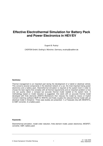
Fig. 11. Comparing the thermal impedance of the reduced model with the original model. Left is thethermal impedance, right is the relative difference between the original and reduced models.AmbientP REFQP8P7P6P5P4P2P3P9P1 1P1 2P1 0P1Thermal DomainMechanicalDomainElectrical Domainz upz vpz wpInduction Motor 20kWU2Simplorer4IN AE1IN BIN CVM311z umz vmR6R5R4AAAOUT AANOUT BBROT1CROT2OUT CR1R2MASS ROT1R3z wm 0VFig. 12. Electrothermal simulation with the IGBT converter in Simplorer5Battery PackIn this section the results from [10] will be presented. The finite element model of a battery pack hasbeen developed by the company Lion Smart in ANSYS [11][12] (see Fig 13). The model consists from32 individual batteries that have been cooled through pipes modeled by means of one dimensionalFLUID116 elements in ANSYS. The finite element model has the dimension roughly 50 000 degreesof freedom and its transient simulation for 100 timesteps takes 40 min.MOR for ANSYS has been employed to reduce the ANSYS model. Again the reduced model with 15degrees of freedom per input was able to approximate the original model with accuracy better than 1%(see Fig. 14). Transient simulation of the reduced model takes less than one second.The coupling of the reduced model with the impedance model of one battery cell is shown in Fig 15.The battery generates power dissipation that is fed to the compact thermal model and at the sametime battery parameters depends on temperature that comes from the thermal model. It is alsopossible to model each battery cell independently. To this end one has to couple more electricalmodels with the thermal model.3. Grazer Symposium Virtuelles Fahrzeug76.-7. Mai 2009Graz, Österreich
Fig. 13. The battery pack model (http://www.lionsmart.de/)Fig. 14. The comparison in Simplorer of the thermal impedance for one load caseFig. 15. Electrothermal simulation of one cell in Simplorer3. Grazer Symposium Virtuelles Fahrzeug86.-7. Mai 2009Graz, Österreich
6ConclusionWe have shown that
As a part of ECPE Tutorial [9], thermal management of an IGBT converter shown in Fig 2 has been performed with ANSYS Icepak. The model has been simplified with the assumption that the heat flow from IGBTs goes only in the direction of the heat sink, that is, the upper surfaces of IGBTs has been considered as adiabatic (see Fig. 8 left). The geometry of semiconductors as well as of the heat .