Transcription
Sains Malaysiana 44(9)(2015): 1363–1370Statistical Analysis of Vehicle Theft Crime in Peninsular Malaysiausing Negative Binomial Regression Model(Analisis Statistik Jenayah Kecurian Kenderaan di Semenanjung Malaysiamenerusi Model Regresi Binomial Negatif)MALINA ZULKIFLI, AHMAD MAHIR RAZALI*, NURULKAMAL MASSERAN & NORISZURA ISMAILABSTRACTThe aim of this paper was to identify the determinants that influence vehicle theft by applying a negative binomialregression model. The identification of these determinants is very important to policy-makers, car-makers and carowners, as they can be used to establish practical steps for preventing or at least limiting vehicle thefts. In addition,this paper also proposed a crime mapping application that allows us to identify the most risky areas for vehicle theft.The results from this study can be utilized by local authorities as well as management of internal resource planning ofinsurance companies in planning effective strategies to reduce vehicle theft. Indirectly, this paper has built ingenuityby combining information obtained from the database of Jabatan Perangkaan Malaysia and insurance companies topioneer the development of location map of vehicle theft in Malaysia.Keywords: Crime; mapping; negative binomial; spatial analysis; vehicle theftABSTRAKTujuan penulisan kertas ini adalah untuk mengenal pasti penentu yang mempengaruhi kecurian kenderaan denganmenggunakan model regresi binomial negatif. Pengenalpastian penentu ini penting kepada pembuat dasar, pembuat keretadan pemilik kereta kerana maklumat ini boleh digunakan untuk mewujudkan langkah-langkah praktikal dalam mencegahatau sekurang-kurangnya menghadkan kejadian kecurian kenderaan. Di samping itu, kertas ini juga mencadangkansuatu aplikasi pemetaan jenayah yang membolehkan kita mengenal pasti kawasan yang paling berisiko untuk berlakunyakecurian kenderaan. Hasil daripada kajian ini boleh digunakan oleh pihak berkuasa tempatan dan juga pihak pengurusanperancangan sumber dalaman syarikat insurans untuk merancang strategi yang berkesan bagi mengurangkan kecuriankenderaan. Secara tidak langsung, kertas kerja ini telah membina satu jalan pintar dengan menggabungkan maklumatyang diperoleh daripada pangkalan data Jabatan Perangkaan Malaysia dan syarikat-syarikat insurans untuk merintiskepada pembinaan peta lokasi kecurian kenderaan di Malaysia.Kata kunci: Analisis reruang; binomial negatif; jenayah; kecurian kenderaan; pemetaanINTRODUCTIONVehicle theft is categorized as a property crime, also knownas a highly organized crime and is one of the many globalissues affecting the world, including Malaysia. Althoughmost stolen vehicles are equipped with security systemsor immobilizers, the number of vehicle theft cases is highand has increased over the years. In Malaysia, there areapproximately 18 million registered vehicles and vehicleowners are required to purchase motor insurance. Statisticsshow that one vehicle was stolen every ten seconds duringthe first nine months of 2007 (Insurance Services MalaysiaBhd 2007). This insurance coverage will protect and paythe vehicle owner if their vehicle is stolen in which casethe insurance covers the loss of the owner based on themarket price of the stolen vehicle.The crime index in Malaysia is defined as the indexof crimes that are reported with sufficient regularityand significance and it is used to quantify crime and toevaluate the effectiveness of crime prevention measures.The crime index in Malaysia can be divided into violentcrimes and property crimes. Although violent crimes attractthe greatest attention of both the public and the media inMalaysia, property crimes accounts for approximately 90%of all crimes reported from 1980 to 2004 and are closelylinked to the total crime index. Approximately 49% of thetotal crime index is attributed to vehicle theft (Sidhu 2005).The identification of the determinants of vehicletheft is important to policymakers, car manufacturers andcar owners because they can indicate possible practicalsteps for preventing or at least limiting, vehicle theft.When predicting the risk of vehicle theft per vehicle,the exposure is the number of vehicles owned and thepossible factors are vehicle use, vehicle model, vehicleage, vehicle location such as residential or business andvehicle geographical location. When relating vehicle theftwith social and economic factors per census block size ordistrict, the exposure is the size of the population which isin term of census block size or district size and the possible
1364factors are population density, average number of personsper household, proportion of the population aged 15-24,proportion of certain races and unemployment rates.Kelly (2000) studied the relationship betweeninequality and crime using a quasi-Poisson regressionmodel. Osgood (2000) analyzed juvenile arrest ratesfor robbery by implementing the Poisson and negativebinomial regression models. Kleck and Chiricos (2002)studied the effect of unemployment on property crimeby fitting the Poisson and negative binomial regressionmodels. Di Tella and Schargrodsky (2004) estimated theeffect of police presence on car theft by implementing theleast squares regression model. Demombynes and Ozler(2005) examined the effects of local inequality on propertyand violent crime in South Africa using the negativebinomial regression model.Aitkin et al. (1990) and Renshaw (1994) used thePoisson regression model for fitting claim count data.Brockman and Wright (1992), Ismail and Jemain (2007)and McCullagh and Nelder (1989) suggested a quasiPoisson regression model to accommodate overdispersionin claim count and count data in other areas. The negativebinomial regression model has been fitted for overdispersedclaim count and count data in other areas by Ismail andJemain (2007), Lawless (1987), McCullagh and Nelder(1989) and Zulkifli et al. (2013). Generalized Poissonregression models have been applied to overdispersed andunderdispersed count data by Consul (1989), Consul andFamoye (1992), Wang and Famoye (1997), Zamani andIsmail (2012) and Zamani and Ismail (2014).Vehicle theft, like most other crime, is spatiallyconcentrated. Crime mapping has become an importanttools in crime and justice. Advances in informationtechnology and software development provide newopportunities for digital mapping to assist crime andprevention programs. Crime mapping is also useful instudying the environmental and geographical aspects ofcrime. Maps allow the areas of unusually high or lowconcentration to be identified visually. However, the mapis only a pictorial representation of the results of complexspatial data analysis.Crime mapping is often thought of as the simpledisplaying and querying of crime data. However, it isa general term that encompasses the technical aspectsof visualization and statistical techniques, as wellas the practical aspects of geographic principles andcriminological theories. In fact, the idea of crime mappingis not new, as it dated back to the early 1800’s in France.A review of the literature from that period to the presentshows several epochs during which interest in crimemapping was high, but then faded dramatically (Weisburd& McEwen 1997). The first map of crime was created byAdriano Balbi and Andre-Michel Guerry in 1829 (Beirne1993; Kenwitz 1987). Using criminal statistics from 1825to 1827 and demographic data from France’s census, theydeveloped maps of crimes against property, crimes againstpersons and levels of education. In recent years, research byDi Tella and Schargrodsky (2004) found a large, negativeand highly local effect of police presence on car theft.Blocks that receive police protection experience 0.081fewer car thefts per month than blocks that do not.In this paper, we proposed an application of thenegative binomial regression model for identifying thedeterminants influencing vehicle theft and an applicationof crime mapping that identifies the riskiest areas forvehicle theft. In the next section, we discuss the materialand methods used in this study, followed by the results anddiscussion sections. The last section is the conclusion.MATERIALS AND METHODSSPATIAL ANALYSISThe Moran’s I test is a test measures the spatialautocorrelation in a random field. Spatial autocorrelationin a random field is the correlation between an observationat region i, yi and an observation at region j, yj. Spatialautocorrelation measures the correlation between thesame attributes at two locations. A positive autocorrelationimplies that observations in close spatial proximity areexpected to be more similar than observations that aremore spatially separated. Conversely, a negative spatialautocorrelation implies that, proximity in space shouldnot provide similar attribute values. The Moran’s I testis calculated as the ratio of the product of the variableof interest and its spatial lag, to the cross product of thevariable of interest, adjusted for the spatial weights used.Its formula is given by:(1)where yi is the observation or attribute value in regioni, is the mean of the variable of interest and wij is thespatial weight of the link between region i and region j.The weight wij assigned to region j, if it is a neighbour ofregion i, can be written as:(2)Inference for I can be derived by using permutationtests, Monte-Carlo tests or approximate tests based on theasymptotic distribution of I. Here, the mean and varianceof I can be derived via the assumption of randomizing theattribute values to the lattice regions. The mean for I viathe assumption of randomizing is given as:(3)The Moran’s I statistic is as follows. If, thespatial autocorrelation is positive and increases in strengthwith and the connected regions tend to have
1365similar attribute values. In contrast, if, the attributevalue of connected regions tends to be dissimilar, whichimplies a negative spatial autocorrelation in a random field(Schabenberger & Gotway 2005).sample size. The probability mass function (pmf) of aPoisson regression model is given by:INVERSE DISTANCE WEIGHTING METHOD (IDW)where the mean and the variance are equal, E(Yi) Var(Yi) μi.To incorporate covariates and to ensure nonnegativity, the mean is included in the Poisson modelthrough a log link function, μi ei exp( β) or ln(μi) ln(e i) , where x ik denotes the explanatoryis a simple method for the spatial estimation of arandom field. IDW is a weighted average interpolator,which can either be an exact or a smoothing interpolator.In IDW, data are weighted during interpolation such that theinfluence of one point relative to another declines as thedistance increases. The value p(Y; s0) at the pivot point socan be estimated by using a weighted mean of the availablemeasurements through the expression.IDW(4)where yi is the observed data for region; i, (si, s0) is thedistance between the centre region i and the pivot points0, and W(si, s0) is the weighting factor that decreases asthe distance increases. Its value decreases with distancefollowing a quadratic or exponential law.The IDW has been recognized as a good method fora spatial interpolation that is based on the knowledgeof distance. For the vehicle theft crime data, we believethat the adjacent region will have similar characteristicsin term of the vehicle theft crime. Thus, it is reasonableto give a large weighted for the adjacent region and asmaller weighted for the regions that have a long distancebetween each other. The interpolation values for thenumber of vehicle theft crime at the unobservable point aredetermined using the observable pair of data accompaniedwith the weighted assigned. Apart from that, although thereare many other methods such as based on the Kriging,triangulation and trend surface, all of these methods haveits own inherent assumptions and strict requirement aboutthe spatial in order to apply it to a real data set. Whilethe IDW does not require any strong assumption, it canalways be a good alternative method in spatial analysis.For example, the Kriging method requires knowledge ofspatial correlation in the random field that is translatedusing the semivariogram model. In our pre-determinedanalysis (not shown in this paper), we have found that thespatial correlation for the number of vehicle theft crime inPeninsular Malaysia cannot be fitted to any of the availablesemivariogram. Consequently, a spatial interpolation basedon Kriging will not provide a good result. Thus, accordingto Hengl (2007) and Masseran et al. (2012a, 2012b), theIDW is a reliable method to overcome this problem.NEGATIVE BINOMIAL REGRESSION MODELSLet (Y1, Y2, , Yn) be the vector of count random variableswhere Yi and Yj are independent for any i j and n is theT(5)variables, βk are the regression parameters, ei is theexposure, xi is the vector of the explanatory variablesand β is the vector of the regression parameters.Under the Poisson distribution, the mean is assumedto be constant or homogeneous within case i, or level i,or cell i. By defining a specific distribution for the mean,heterogeneity within cases is allowed. Assuming Yi λi isdistributed as a Poisson with conditional mean E(Yi λi) λi, λi is distributed as a gamma with mean E(λi) μi andvariance is Var(λi) μi2vi-1, the marginal distribution of Yifollows a negative binomial with pmf;(6)where the mean is E(Yi) μi and the variance is Var(Yi) μi(1 μivi-1). When vi a-1, the negative binomialdistribution is produced, with mean E(Yi) μi and varianceVar(Yi) μi(1 aμi). The pmf (Cameron & Trivedi 1986;Lawless 1987) is(7)where a denotes the dispersion parameter. If a equalsto zero, the mean and the variance are equal; if a 0,the variance exceeds the mean and the NB allows foroverdispersion.If the mean is assumed to follow a log link function,μi ei exp( β), the log likelihood for the NB regressionmodel can be written asln L(β, a) (8)The maximum likelihood estimates for the negativebinomial regression model can also be obtained bymaximizing ln L(β, a) with respect to β and a.
1366LIKELIHOOD RATIO TEST, WALD TEST, AIC AND BICThe test of overdispersion in the NB regression modelscan be assessed using the likelihood ratio test becauseNB regression reduces to Poisson regression in the limitwhen a 0. The hypothesis are H0 : a 0 against H1 :a 0 which is a one-sided test. The likelihood ratio is T 2(ln L1 – ln L0), where ln L1 and ln L0 are the model’slog likelihood under the respective hypothesis. Since thenull hypothesis is on the boundary of parameter space, Thas an asymptotic distribution of probability mass of 0.5at zero and 0.5 of chi-square distribution with one degreeof freedom. In other words, to test the null hypothesisat significance level α, the critical value of chi-squaredistribution with significance level 2α is used, or reject H0if T . As an example, for 0.05 significance level, thecritical value is 2.705 instead of 3.8415.The test of overdispersion in the negative binomialregression model can also be performed by the Waldstatistic, which is defined as the ratio of the estimatedoverdispersion parameter to its standard error,where asymptotically, the statistic follows a standardnormal distribution.One can also compare the performance of alternativemodels based on several likelihood measures, such asthe Akaike Information Criteria (AIC) and the BayesianSchwartz Information Criteria (BIC). The AIC penalises amodel with a larger number of parameters and is definedas AIC –2 ln L 2p, where ln L denotes the fitted loglikelihood and p is the number of parameters. The BICpenalises a model with a larger number of parametersand a larger sample size and is defined as BIC –2 ln L p ln(n), where n is the sample size. The best model isindicated by the smallest AIC and BIC.RESULTSDATACrime data for private car theft were obtained and compiledfrom insurance companies in Malaysia. In particular,automobile theft insurance indemnifies the insured againstthe loss of a motor vehicle through theft. The data are from2001 to 2003 and were supplied by Insurance ServicesMalaysia (ISM).Population data on the social and economicbackground of each district were obtained and compiledfrom the Malaysian 2000 census data, supplied by JabatanPerangkaan Malaysia. The data provide information on81 districts of all 11 states in Peninsular Malaysia. Thedistrict population ranges from 11,183 to 1,305,792 withan average of 163,856.Table 1 shows the demographic and sociologicalfactors considered for the independent (explanatory)variables. Further explanations on the demographic andsocial factors in Table 1 are as follow:TABLE1. Demographic and sociological factorsfor vehicle theft essModerateHighIndia1.2.3.LessModerateHighOthers :1.2.3.LessModerateHighForeign migrants1.2.3.LessModerateHighProfessional :1.2.3.LessModerateHighWork :1.2.3.LessModerateHighProductivity1.2.3.Not productiveProductiveVery productivePolice station1.2.3.LessModerateHighPopulation densityPopulation density Population density is defined asnumber of population per km2. Population density isdivided into three quantiles; low, medium and highGender Gender is divided into two proportions; maleand femaleBumiputra Bumiputra is defined as number of bumiputraper 1000 population. This factor is divided into threequantiles; less, moderate and highChinese Chinese is defined as number of chinese per 1000population. This factor is divided into three quantiles; less,moderate and highIndian Indian is defined as number of indian per 1000population. This factor is divided into three quantiles; less,moderate and high
1367Others Others is defined as the number of other races(besides bumiputra, chinese and indian) per 1000population. This factor is divided into three quantiles; less,moderate and highForeign migrant Foreign migrant is defined as numberof foreign migrant per 1000 population. Foreign migrantis divided into three quantiles; less, moderate and highProfessional Professional is defined as number ofprofessional workers per 1000 population. Professionalis divided into three quantiles; less, moderate and highWork Work is defined as number of working employeeper 1000 population. Work is divided into three quantiles;less, moderate and highProductivity Productivitiy is defined as productivityper 1000 population. Productivity is divided into threequantiles; not productive, productive and very productivePolice station Police station is defined as number of policestation per 1000 populatio. Police station is divided intothree quantiles; less, moderate and highTABLE2. Estimated parameters for negative binomial regression modelParameterInterceptDensity :Gender :Bumiputra :Chinese :India :Others :Foreign migrants :Professional :Work :Productivity :Police station :Log likelihoodAICBICRESULTS ON NEGATIVE BINOMIAL REGRESSION ANALYSISIn determining the factors that influence the occurrenceof vehicle theft in certain areas, independent variables(explanatory variables) for each district are analysed. Inthis study, negative binomial regression is used to modelthe relationship between the explanatory variables withthe number of burglaries in the district, where populationis used as offset.Table 2 shows the parameters, log likelihood, AICand BIC for the fitted regression model. Based on thep-value, the results indicated that high population densityis a significant factor in the occurrence of vehicle theft.Thus, the district with higher population density tendsto have more cases of car theft. It also appears that thenumber of police stations in a district has a significanteffect on the rate of car thefts in the area. However, racialcomposition, foreign migration, productivity, number ofworkers and number of professional employees do notplay an important role in influencing the rate of car theftin any district.Table 3 shows the parameters, log likelihood, AICand BIC for the negative binomial regression model withcovariates that are significant at 5% level. It appears thatpopulation density, Chinese composition and the 437less-1.0616-2.760productivevery 9-2.041-269.943559.286583.830***, ** and * indicates that the parameters are significant at 0.01, 0.05 and 0.10 levels, 760.6680.0060.041***
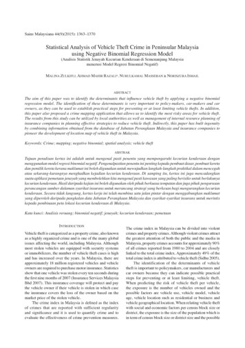
1368of police stations is significant factors contributing to thecar theft rate in the districts of Peninsular Malaysia.with many industrial activities and locations of tourismattraction.RESULTS ON SPATIAL ANALYSISDISCUSSIONFigure 1 shows the population density of the districts ofPeninsular Malaysia. The darkest area indicates the districtwith the highest population density.Figure 2 shows the map of vehicle theft in districtsof Peninsular Malaysia based on the negative binomialregression model shown in Table 3. The darkest area onthe map has the highest rate of car theft. As shown, areaswith high rate of car theft are Klang Valley, Johor Bahruand Penang, which are areas of high population density,TABLEThis paper builds an initiative by combining the informationfrom Jabatan Perangkaan Malaysia and insurance companiesto pioneer the creation of map of vehicle theft locationin Peninsular Malaysia. The map and the accompanyinganalyses will help policymakers to classify districts andidentify primary factors regarding vehicle theft. Theseinformation can also be supplied to local authorities andmanagement of resource planning department of insurancecompanies for planning strategies of reducing car theft.3. Negative binomial regression model with significant covariatesParameterInterceptDensity :Chinese :Police station :Log 7**0.0000.000***, ** and * indicates that the parameters are significant at 0.01, 0.05 and 0.10 levels, respectivelyFIGURE1. Map of population density in districts of Peninsular Malaysia*********
1369FIGURE2. Map of vehicle theft in districts of Peninsular Malaysiabased on negative binomial regression modelThere are several preventive and corrective measuresthat can be implemented by manufacturers to reduce thenumber of stolen vehicles such as anti-theft alarms andanti-theft key locks. Property managers may also assist byproviding protected and secured parking, as well as hiringsecurity guards.The Royal Malaysian Police may also strategize inincreasing the number of police stations and locatingthem in strategic and dangerous areas, especially in theareas that show large numbers of reported vehicle thefts.A study on the existence of anti-theft devices and securedparking, as well as the number and the location of thepolice stations, can be carried out if information on thesefactors is provided in police reports (for the number ofstolen vehicles), insurance claim reports (for the number ofvehicle theft claims) or insurance policies (for the numberof vehicle exposures). That information can be embeddedin a regression model by using the contributing factors ascovariates.ACKNOWLEDGEMENTSThis research is financed by the Fundamental ResearchGrant Scheme (Code: FRGS/1/2011/ST/UKM/02/8).REFERENCESAitkin, M., Anderson, D., Francis, B. & Hinde, J. 1990. StatisticalModelling in GLIM. New York: Oxford University Press.Beime, P. 1993. Inventing Criminology. Albany, NY: StateUniversity of New York Press.Brockmann, M.J. & Wright, T.S. 1992. Statistical motor rating:making effective use of your data. Journal of the Institute ofActuaries 119(3): 457-543.Cameron, A.C. & Trivedi, P.K. 1986. Econometric modelsbased on count data: Comparisons and applications of someestimators and tests. Journal of Applied Econometrics 1:29-53.Consul, P.C. 1989. Generalized Poisson Distribution: Propertiesand Application. New York: Marcel Dekker.Consul, P.C. & Famoye, F. 1992. Generalized Poissonregression model. Communications in Statistics (Theory &Methodology) 2(1): 89-109.Demombynes, G. & Ozler, B. 2005. Crime and local inequalityin South Africa. Journal of Development Economics 76:265-292.Di Tella, R. & Schargrodsky, E. 2004. Do police reduce crime?Estimates using the allocation of police forces after a terroristattack. The American Economic Review 94(1): 115-133.Hengl, T. 2007. A Practical Guide to Geostatistical Mappingof Environmental Variables. Italy: European Communities.
1370Insurance Services Malaysia Bhd. 2007. Insurance industrystatistics on stolen vehicles. http://www.piam.org.my/news/piamnews/p014.htm. Accessed 22 June 2011.Ismail, N. & Jemain, A.A. 2007. Handling overdispersion withnegative binomial and generalized Poisson regression models.Casualty Actuarial Society Forum Winter. pp. 103-158.Kelly, M. 2000. Inequality and crime. The Review of Economicsand Statistics 82(4): 530-539.Kenwitz, J.W. 1987. Cartography in France: 1660-1848.Chicago, IL: University of Chicago Press.Kleck, G. & Chiricos, T, 2002. Unemployment and propertycrime: A target-specific assessment of opportunity andmotivation as mediating factors. Criminology 40(3): 649-680.Lawless, J.F. 1987. Negative binomial and mixed Poissonregression. Canadian Journal of Statistics 15(3): 209-225.Masseran, N., Razali, A.M. & Ibrahim, K. 2012a. An analysisof wind power density derived from several wind speeddensity functions: The regional assessment on wind powerin Malaysia. Renewable and Sustainable Energy Reviews16(8): 6476-6487.Masseran, N., Razali, A.M., Ibrahim, K., Zin, W.Z.W. & Zaharim,A. 2012b. On spatial analysis of wind energy potential inMalaysia. WSEAS Transactions on Mathematics 11(6):467-477.McCullagh, P. & Nelder, J.A. 1989. Generalized Linear Models.2nd ed. London: Chapman and Hall.Osgood, W. 2000. Poisson-based regression analysis of aggregatecrime rates. Journal of Quantitative Criminology 16: 21-43.Renshaw, A.E. 1994. Modelling the claims process in the presenceof covariates. ASTIN Bulletin 24(2): 265-285.Schabenberger, O. & Gotway, C.A. 2005. Statistical Methodsfor Spatial Data Analysis. Boca Raton: Chapman & Hall/CRC Press.Sidhu, A.S. 2005. The rise of crime in Malaysia: An academicand statistical analysis. Journal of the Kuala Lumpur RoyalMalaysia Police College 4: 1-28.Wang, W. & Famoye, F. 1997. Modeling household fertilitydecisions with generalized Poisson regression. Journal ofPopulation Economics 10: 273-283.Weisburd, D. & McEwen, T. 1997. Introduction: Crime Mappingand Crime Prevention. Monsey, NY: Criminal Justice Press.Zamani, H. & Ismail, N. 2012. Functional form for the generalizedPoisson regression model. Communications in Statistics Theory and Methods 41(20): 3666-3675.Zamani, H. & Ismail, N. 2014. Functional form for thezero-inflated generalized Poisson regression model.Communications in Statistics - Theory and Methods 43(3):515-529.Zulkifli, M., Ismail, N. & Razali, A.M. 2013. Analysis of vehicletheft: A case study in Malaysia using functional forms ofnegative binomial regression models. Applied Mathematicsand Information Sciences 7(2L): 389-395.Malina ZulkifliSchool of Quantitative Sciences, College of Arts and ScienceUniversiti Utara Malaysia06010 Sintok, Kedah Darul AmanMalaysiaAhmad Mahir Razali* , Nurulkamal Masseran & Noriszura IsmailSchool of Mathematical SciencesFaculty of Science and TechnologyUniversiti Kebangsaan Malaysia43600 Bangi, Selangor Darul EhsanMalaysia*Corresponding author; email: mahir@ukm.edu.myReceived: 17 June 2014Accepted: 20 May 2015
and highly local effect of police presence on car theft. Blocks that receive police protection experience 0.081 fewer car thefts per month than blocks that do not. In this paper, we proposed an application of the negative binomial regression model for identifying the determinants influencing vehicle theft and an application of crime mapping that identifies the riskiest areas for vehicle theft .