Transcription
Ecological Modelling 244 (2012) 57–64Contents lists available at SciVerse ScienceDirectEcological Modellingjournal homepage: www.elsevier.com/locate/ecolmodelReviewSpecies detection vs. habitat suitability: Are we biasing habitat suitability modelswith remotely sensed data?Bethany A. Bradley a, , Aaryn D. Olsson b , Ophelia Wang b , Brett G. Dickson b , Lori Pelech a ,Steven E. Sesnie b , Luke J. Zachmann babDepartment of Environmental Conservation, University of Massachusetts, Amherst, MA 01003, United StatesLab of Landscape Ecology and Conservation Biology, School of Earth Sciences and Environmental Sustainability, Northern Arizona University, Flagstaff, AZ 86011, United Statesa r t i c l ei n f oArticle history:Received 2 April 2012Received in revised form 13 June 2012Accepted 18 June 2012Keywords:Bioclimatic envelope modelEcological niche modelHabitat suitability modelLand cover classificationRemote sensingSpecies distribution modelVegetationa b s t r a c tRemotely sensed datasets are increasingly being used to model habitat suitability for a variety of taxa.We review habitat suitability models (HSMs) developed for both plants and animals that include remotesensing predictor variables to determine how these variables could affect model projections. For modelsfocused on plant species habitat, we find several instances of unintentional bias in HSMs of vegetationdue to the inclusion of remote sensing variables. Notably, studies that include continuous remote sensingvariables could be inadvertently mapping actual species distribution instead of potential habitat due tounique spectral or temporal characteristics of the target species. Additionally, HSMs including categoricalclassifications are rarely explicit about assumptions of habitat suitability related to land cover, whichcould lead to unintended exclusion of potential habitat due to current land use. Although we supportthe broader application of remote sensing in general, we caution developers of HSMs to be aware ofintroduced model bias. These biases are more likely to arise when remote sensing variables are addedto models simply because they improve accuracy, rather than considering how they affect the modelresults and interpretation. When including land cover classifications as predictors, we recommend thatmodellers provide more explicit descriptions of how habitat is defined (e.g., is deforested land consideredsuitable for trees?). Further, we suggest that continuous remote sensing variables should only be includedin habitat models if authors can demonstrate that their inclusion characterizes potential habitat ratherthan actual species distribution. Use of the term ‘habitat suitability model’ rather than ‘species distributionmodel’ could reduce confusion about modelling goals and improve communication between the remotesensing and ecological modelling communities. 2012 Elsevier B.V. All rights reserved.Contents1.2.3.4.5.6.Introduction . . . . . . . . . . . . . . . . . . . . . . . . . . . . . . . . . . . . . . . . . . . . . . . . . . . . . . . . . . . . . . . . . . . . . . . . . . . . . . . . . . . . . . . . . . . . . . . . . . . . . . . . . . . . . . . . . . . . . . . . . . . . . . . . . . . . . . . . . .Terminology . . . . . . . . . . . . . . . . . . . . . . . . . . . . . . . . . . . . . . . . . . . . . . . . . . . . . . . . . . . . . . . . . . . . . . . . . . . . . . . . . . . . . . . . . . . . . . . . . . . . . . . . . . . . . . . . . . . . . . . . . . . . . . . . . . . . . . . . . .Remotely sensed data as predictors of animal habitat suitability . . . . . . . . . . . . . . . . . . . . . . . . . . . . . . . . . . . . . . . . . . . . . . . . . . . . . . . . . . . . . . . . . . . . . . . . . . . . . . . . . . .Remotely sensed data as predictors of plant habitat suitability . . . . . . . . . . . . . . . . . . . . . . . . . . . . . . . . . . . . . . . . . . . . . . . . . . . . . . . . . . . . . . . . . . . . . . . . . . . . . . . . . . . .4.1.The chicken and egg problem: do trees only grow in forests? . . . . . . . . . . . . . . . . . . . . . . . . . . . . . . . . . . . . . . . . . . . . . . . . . . . . . . . . . . . . . . . . . . . . . . . . . . . . . .4.2.Mistaking actual species distribution for potential species distribution . . . . . . . . . . . . . . . . . . . . . . . . . . . . . . . . . . . . . . . . . . . . . . . . . . . . . . . . . . . . . . . . . . . .4.3.Sacrificing at the altar of accuracy . . . . . . . . . . . . . . . . . . . . . . . . . . . . . . . . . . . . . . . . . . . . . . . . . . . . . . . . . . . . . . . . . . . . . . . . . . . . . . . . . . . . . . . . . . . . . . . . . . . . . . . . . . .Recommendations for remote sensing in habitat suitability models . . . . . . . . . . . . . . . . . . . . . . . . . . . . . . . . . . . . . . . . . . . . . . . . . . . . . . . . . . . . . . . . . . . . . . . . . . . . . . .Conclusions . . . . . . . . . . . . . . . . . . . . . . . . . . . . . . . . . . . . . . . . . . . . . . . . . . . . . . . . . . . . . . . . . . . . . . . . . . . . . . . . . . . . . . . . . . . . . . . . . . . . . . . . . . . . . . . . . . . . . . . . . . . . . . . . . . . . . . . . . .Acknowledgment . . . . . . . . . . . . . . . . . . . . . . . . . . . . . . . . . . . . . . . . . . . . . . . . . . . . . . . . . . . . . . . . . . . . . . . . . . . . . . . . . . . . . . . . . . . . . . . . . . . . . . . . . . . . . . . . . . . . . . . . . . . . . . . . . . . .References . . . . . . . . . . . . . . . . . . . . . . . . . . . . . . . . . . . . . . . . . . . . . . . . . . . . . . . . . . . . . . . . . . . . . . . . . . . . . . . . . . . . . . . . . . . . . . . . . . . . . . . . . . . . . . . . . . . . . . . . . . . . . . . . . . . . . . . . . . . Corresponding author at: 160 Holdsworth Way, Amherst, MA 01003, United States. Tel.: 1 413 545 1764; fax: 1 413 545 4358.E-mail address: bbradley@eco.umass.edu (B.A. Bradley).0304-3800/ – see front matter 2012 Elsevier B.V. All rights 2.06.0195858596060606262626363
58B.A. Bradley et al. / Ecological Modelling 244 (2012) 57–641. IntroductionRemotely sensed data are widely recognized for their applicability to ecological research (Kerr and Ostrovsky, 2003; Pettorelli et al.,2005). Ecological applications of remotely sensed data include classification and quantification of land features, modelling ecosystemfunction (e.g., to predict net primary productivity), and mappingland cover change (e.g., to identify habitat loss or afforestation)(Kerr and Ostrovsky, 2003). Remotely sensed data have also beenused as a proxy for species richness and biodiversity (Gillespie et al.,2008; Turner et al., 2003). As remotely sensed datasets are more frequently and readily available, including the Landsat image archive(Woodcock et al., 2008) and moderate resolution imaging spectroradiometer (MODIS) phenology products (Tan et al., 2011), it islikely that ecological modellers and biogeographers will continueto expand their use of remotely sensed data.Habitat suitability modelling in particular has seen considerable recent growth in the application of remotely sensed data.Habitat suitability models (HSMs; also termed species distributionmodels, ecological niche models, or bioclimatic envelope models)use empirical relationships between a species’ distribution andenvironmental variables (e.g., climate, topography, and soils) topredict potential suitable habitats across a landscape or region(Franklin, 1995; Guisan and Zimmermann, 2000). Applications ofHSMs include ecological reserve planning (e.g., Kremen et al., 2008),prediction of non-native species invasions (e.g., Thuiller et al.,2005), and risk assessments for native species (e.g., Thomas et al.,2004). Remotely sensed data can directly measure, or serve asa proxy for variables that affect habitat suitability. As a result,including remotely sensed data as variables can improve the overall accuracy of predictive models, making them attractive for usein HSMs (Bradley and Fleishman, 2008; Leyequien et al., 2007;Pettorelli et al., 2011).Species habitat is affected by a range of environmental variables at varying scales. At regional to continental scales, suitabilityis most influenced by climate while, at landscape scales, climatesuitability is modified by land use, land cover and topography.Suitability is further modified at local scales by soil conditionsand micro-topography (Pearson and Dawson, 2003). Unfortunately,continuous spatial measurements of these environmental variables can be difficult to acquire, and many environmental variablesare increasingly derived from remotely sensed data. Examples ofthese products include the normalized difference vegetation index(NDVI) as a proxy for ecosystem greenness (Fig. 1), the shuttle radartopography mission (SRTM) for high resolution topographic data,and emerging light detection and ranging (LIDAR) data as a proxyfor vegetation community structure (for more details on these andother remote sensing products, see Gillespie et al., 2008; Pettorelliet al., 2005).Remotely sensed measures of vegetation productivity (e.g.,NDVI, enhanced vegetation index—EVI) and biophysical parameters (leaf area index—LAI) have been used extensively as predictorsof habitat characteristics for animals (Pettorelli et al., 2011). However, a number of recent studies have applied vegetation proxiesor land cover data to models of plant species habitat (Table 1).Unfortunately, the potential benefit of these remotely sensed datain HSMs constructed for plants is less clear. Plant habitat modelscould be biased by remotely sensed measures of vegetation likeNDVI, resulting in outcomes that underestimate the species’ potential distribution due to correlations between species distributionand spatial patterns identified by remote sensing. Remotely sensedproxies for vegetation could also highlight disturbed areas or otherspatially heterogeneous patterns (e.g., recent precipitation historyin arid lands; Fig. 2) that are poorly linked to habitat suitability.In this context, we review remote sensing applications forhabitat suitability modelling, briefly covering novel applicationsFig. 1. Phenological metrics derived from time series of remotely sensed vegetation indices (e.g., NDVI) could provide novel predictor variables for animal and planthabitat models (Tan et al., 2011). (A) Example phenology metrics derived from single year or annual average vegetation phenology. Start of season (SOS) and end ofseason (EOS) are in this case based on the time when overall ecosystem greenness reaches half of its maximum value. (B) Example time series showing highinter-annual variability in vegetation productivity, potentially a predictor of habitat.for animal habitat modelling (reviewed comprehensively byLeyequien et al., 2007; Pettorelli et al., 2011), and then focusingon the use (and possible misuse) of remotely sensed variables forplant habitat modelling.2. TerminologyThe science of habitat modelling based on empirical relationships between species distribution and spatially explicitenvironmental variables suffers from numerous near-synonymousterms (see Franklin, 2009 for a full discussion). One of the mostwidely used terms is species distribution model (SDM), which isgenerally understood by the ecological modelling community tomean a model of potential species distribution.Unfortunately, this term in particular can cause confusionamongst the remote sensing community because remote sensing typically focuses on modelling the actual species distribution(e.g., Kerr and Ostrovsky, 2003; Xie et al., 2008). Remote sensingstudies might aim to model the distribution of individual plantspecies (termed ‘species mapping’, Nagendra, 2001), while othersmodel the distribution of dominant vegetation types (termed ‘landcover classification, Kerr and Ostrovsky, 2003; Xie et al., 2008).Hence, there is a strong potential for confusion when terminology is poorly defined. Note, however, that there is less potentialfor confusion in animal studies because remotely sensed data arenever used to detect actual animal distribution, only plant distribution. In this review, we will instead use the term habitat suitabilitymodel (HSM) to describe empirical models of potential species
B.A. Bradley et al. / Ecological Modelling 244 (2012) 57–6459Table 1Reference list of habitat suitability models for plants that include remotely sensed variables.Remotely sensed predictor variablesTarget speciesReferencesSpectrally homogenous land cover classification based onLandsatEuropean land cover (PELCOM) from AVHRR aggregated to50 kmLand cover of Britain (2000) & automated land cover mapderived from LandsatASTER-based classification of snow coverMODIS-derived phenology metrics based on NDVI and EVIMODIS NDVI for summer-fall of 2000NDVI, wetness index, temperature, and soil brightnessderived from LandsatMODIS LAI, veg moisture from Qscat and MODIS NDVIDyers woad (Isatis tinctoria)Dewey et al. (1991)European tree speciesThuiller et al. (2004)Four plant species: Rhynchospora alba, Erica tetralix,Salix herbacea & Geranium sylvaticum.Arctic dwarf shrub (Dryas octopetala)Tamarisk (Tamarix spp.)Purple loosestrife (Lythrum salicaria)19 trees in the Great Basin, USAPearson et al. (2004)Three Amazon trees: Calophyllum brasiliensis, Carapaguianensis, Virola surinamensisFive widespread commercial timber treesPrates-Clark et al. (2008)Saatchi et al. (2008)Pine (Pinus spp.) and white oak (Quercus spp.)Cord et al. (2009)Dalmatian toadflax, Musk thistle, Cheatgrass, Whitesweet cloverRare tree: Pittosporum eriocarpumStohlgren et al. (2010)Padalia et al. (2010)Twenty-nine palm species in AfricaBlach-Overgaard et al. (2010)Tamarisk (Tamarix spp.)Two central American trees: Broumum alicastrum andLiquidambar macrophyllaTamarisk (Tamarix spp.)Rosa rubiginosa in ArgentinaGeneralist shrub species in SpainCord et al. (2010)Cord et al. (2011)QSCAT backscatter for canopy roughness and MODIS LAIphenology metricsMODIS phenology metrics derived in house from 2001 to2007 time seriesMODIS phenology metrics, tree coverForest type classes based on visual interpretation ofsatellite imageryGlobal land cover 2000, % tree cover in 2001, AVHRRaverage NDVI 1985–1988MODIS EVI and land surface temperatureMODIS phenology metricsMODIS mean EVI and annual range of EVILandsat NDVI, greenness and brightness indicesLandsat spectral indices and NDVIBeck et al. (2005)Morisette et al. (2006)Anderson et al. (2006)Zimmermann et al. (2007)Jarnevich et al. (2011)Zimmermann et al. (2011)Morán-Ordóñez et al. (2012)Fig. 2. Three Landsat TM colour composite images (bands 4, 3 and 2) of the Sierra Pinacate in northern Sonora, Mexico, each acquired in early September. Red colours identifyareas with actively growing vegetation (similar to high NDVI) in a hot desert environment where precipitation drives phenology. The spatially heterogeneous patterns arecaused by asynchronous plant growth due to isolated rainfall events. If used in a habitat suitability model, the model prediction could vary considerably depending oninter-annual variability (Fig. 1B). (For interpretation of the references to colour in this figure legend, the reader is referred to the web version of the article.)distribution based on environmental correlates (which mightinclude remotely sensed data).3. Remotely sensed data as predictors of animal habitatsuitabilityThere are numerous examples of remote sensing variables beingtested and applied to animal habitat modelling (Leyequien et al.,2007; Pettorelli et al., 2011; Vierling et al., 2008). In many (butnot all) cases, the addition of remotely sensed data improves theaccuracy of the habitat model (Pettorelli et al., 2011). In most ofthese studies, remote sensing variables serve as proxies for vegetation (e.g., structure, composition, and land cover change) or otherattributes of habitat quality. For example, Willems et al. (2009)used NDVI to model habitat of the vervet monkey in Africa, withareas of high NDVI acting as a proxy for food availability and lowvisibility for predators. Bergen et al. (2007) used biomass measurements derived from RADAR to model North American bird habitat,with RADAR-derived biomass acting as a proxy for forest structure.Peterson et al. (2006) used time series of land cover classificationsto model corvid habitat in Mexico, with changes in land cover actingas a proxy for habitat loss.The use of NDVI or land cover classifications in conjunction withclimatic variables often does not improve habitat models becausethese variables can be highly collinear, particularly at regionalscales (e.g., Thuiller et al., 2004; Zimmermann et al., 2007). Remotesensing variables have the greatest potential benefit when theyprovide information distinct from climate. This may occur in areasof broadly similar climate where other features such as soils or disturbance alter vegetation characteristics. In other cases, remotelysensed vegetation indices could be more reflective of climate conditions than interpolated climate because weather stations arehundreds of kilometres apart (e.g., the Amazon; Saatchi et al., 2008).In addition to vegetation indices, other novel remote sensing products and techniques are promising for habitat modelling.Technological and scientific advances have created new proxiesfor vegetation characteristics that are quite distinct from climate:RADAR/LIDAR-based vegetation structure and temporal patterns of
60B.A. Bradley et al. / Ecological Modelling 244 (2012) 57–64vegetation phenology. High-resolution (e.g., 5 m pixel) RADAR andLIDAR measurements are increasingly being used to characterizethree-dimensional vegetation community structure (Bergen et al.,2009; Vierling et al., 2008). RADAR and LIDAR are active sensors,whereby a long-wavelength or laser pulse is directed at the Earth’ssurface. The returned waveform or coordinates can be used to estimate detailed horizontal and vertical vegetation attributes, such asforest canopy height and aboveground biomass (Lefsky et al., 2002).In one example application, Buermann et al. (2008) used RADARsensitivity to estimate canopy roughness at 1 km resolution as apredictor of bird habitat in the Amazon. The National Aeronauticsand Space Administration (NASA) is likely to launch a RADAR satellite aimed at measuring ecosystem structure in 2016 (DESDynI),while the European Space Agency (ESA) will launch the RADARmission Sentinel-1 in 2013. Meanwhile, state-wide airborne LIDARdata are becoming more readily available (e.g., Asner et al., 2011).A second novel predictor of vegetation characteristics that contribute to animal habitat suitability is phenology, or the annual andinter-annual timing of biological events. Average annual phenologyis broadly correlated with climate, particularly start of season withtemperature (e.g., Stöckli and Vidale, 2004), and may serve as aclimate proxy in poorly gaged areas. Spatial variation in phenologycan identify differential responses, even within similar ecosystems,that could affect habitat quality (e.g., Fisher and Mustard, 2007;Morisette et al., 2009), while inter-annual phenology can serve asan indicator of vegetation variability, which may be important forlong-lived animals. Phenological metrics, typically derived fromNDVI time series, include start of season, length of growing season, and inter-annual variability (Tan et al., 2011) (Fig. 1). As apredictor of animal habitat, vegetation phenology has been, forexample, correlated with mosquito life cycles resulting in malariaoutbreaks in Africa (Rogers et al., 2002), habitat of Great Bustardsin Spain (Osborne et al., 2001) and moose body mass in Norway(Herfindal et al., 2006). Newly available phenology metrics derivedfrom high temporal resolution imagery such as MODIS (Tan et al.,2011) at 250 m to 1 km resolution and advanced very high resolution radiometer (AVHRR; http://phenology.cr.usgs.gov/index.php)at 1–8 km resolution should increase the applications of this potential predictor in animal habitat modelling.4. Remotely sensed data as predictors of plant habitatsuitabilityAlthough remotely sensed variables are widely used to modelanimal habitat (Leyequien et al., 2007; Pettorelli et al., 2011), thepractice has been less common in models of plant habitat. However,applications for plant habitat modelling are on the rise (Table 1).Modelling plant habitat requires more care because remotelysensed variables and land cover classifications often directly measure the attributes of the same plant species whose habitat themodel aims to predict. This point seems to be underappreciatedin plant habitat modelling. Below, we review potential sources ofbias that remotely sensed data can introduce into HSMs, and howthey have been handled (or mishandled) in recent research.4.1. The chicken and egg problem: do trees only grow in forests?Are forests the only locations that should be defined as potential tree habitat? The answer to this question lies at the heart ofwhether and how land cover classifications and continuous variables should act as proxies for vegetation cover (e.g., NDVI) andbe used to predict plant and animal habitat suitability. If distribution data occur only in currently forested areas (recently collecteddata are more likely to reflect current land use/land cover patterns),then including these variables will effectively exclude presently‘non-forested’ land from potential habitat. For example, PratesClark et al. (2008) use leaf area index (LAI) and RADAR as predictorvariables for habitat of three rare Amazon trees. The use of LAI inthis instance excluded deforested lands, which had low LAI values.Similarly, by including NDVI in habitat suitability models, Cord et al.(2009) exclude agriculture, urban, and degraded lands from potential habitat for pine and oak species in Mexico. In both of thesecases, the model of suitable tree habitat excludes human modifiedlandscapes. This assumes that potential tree habitat is defined relative to current land use, but the assumption is never made explicit.If currently deforested or non-forested areas are considered to beunsuitable for tree species, then these areas should be excludedprior to further analysis.Conversely, Zimmermann et al. (2011) use remote sensingderived brightness and greenness indices to detect forest clearanceas a predictor of the invasive shrub Rosa rubiginosa in Argentina.In this case, the authors are explicit about their definition of habitat suitability (or invasibility) as stemming directly from existingland clearing and disturbance. The specific interpretation of remotesensing variables in Zimmermann et al. (2011) makes the resulting model more readily understandable and applicable to invasiveplant management.The same problem of defining habitat relative to current landcover potentially applies to any use of land cover classifications,even in the absence of anthropogenic factors. For example, Thuilleret al. (2004) note that modelled habitat suitability for the European tree Quercus petraea is positively associated with percentageforest cover (derived from land cover classifications). Similarly, themodelled habitat of the rare tree Pittosporum eriocarpum in Indiais best described by including forest composition classes (Padaliaet al., 2010). In these examples, the resulting habitat models willbe biased towards current forest, and away from currently nonforested land, suggesting that climatically suitable non-forest isunsuitable habitat for trees.To overcome this ‘chicken and egg’ problem, habitat suitabilitymodelling efforts that include land cover classifications (or proxiesfor land cover) should be explicit about their goals and applications, and discuss how the inclusion of land cover classes influencestheir interpretation. For example, Pearson et al. (2004) argue that byincluding land cover in a habitat model of the flower Erica tetralix,they were able to differentiate between range contraction causedby climate and range contraction caused by land use. Beck et al.(2005) use a remote sensing based classification of snow coverto exclude habitat for the Arctic shrub Dryas octopetala, whichdoes not grow if the climate is moist enough to produce snow.Morán-Ordóñez et al. (2012) show that current land cover limits ageneralist species more than climate alone. In all of the above examples, the authors provide a clear interpretation of how the inclusionof remotely sensed variables alters their models of habitat.4.2. Mistaking actual species distribution for potential speciesdistributionThe use of continuous remote sensing variables (e.g., spectralbands, NDVI, LAI) can be a problem if these variables act as proxies for land cover (see previous section), or if they are sensitiveto unique spectral or temporal properties of the target speciesitself (Fig. 3). This is of particular concern if the target species iscommon, grows in patches with high abundance that could bedetected remotely, or has a unique phenology (e.g., Bradley andMustard, 2005; Tuanmu et al., 2010). For example, Zimmermannet al. (2007) used time series of Landsat-derived NDVI to develophabitat models for 19 tree species across a Utah landscape at90 m spatial resolution. The 19 species ranged from rare to common, but those for which habitat models were most improvedusing remote sensing were broadleaf, deciduous species that are
B.A. Bradley et al. / Ecological Modelling 244 (2012) 57–6461Fig. 3. (A) Aerial photograph taken near Tucson, AZ, which is undergoing invasion by Pennisetum ciliare. The mapped boundary of a large and dynamically expanding patchis shown in outline. Because of its cold intolerance, P. ciliare tends to colonize south-facing slopes in this part of its range. Inset shows this location in relation to the stateof Arizona, USA. (B) NDVI of the invasion site is higher than on neighbouring south-facing slopes due to denser cover of P. ciliare. But, NDVI is similar to surrounding, moreheavily vegetated north-facing slopes where P. ciliare is rare or absent. (C) Habitat suitability model of P. ciliare derived from topographic variables (elevation, slope, aspect)using presence and absence data collected throughout the area and based on a Random Forest regression tree model (Breiman, 2001). Note that areas of highest suitability(light shades) are associated with south-facing slopes. This model explained 2.6% of the variance. (D) Habitat suitability model of P. ciliare derived from topographic variablesplus NDVI. Because NDVI acts as a proxy for species actual distribution, the predicted suitability model identifies only areas where P. ciliare is already present, yet P. ciliarehas been doubling in area at this site every 2–5 years since 1989 (Olsson et al., 2012). This model explained 38.1% of the variance (an “improvement” of model accuracy).easier to discriminate using multi-temporal satellite data becauseof their seasonal phenology. This is one example of including a predictor variable that models actual species distribution rather thanpotential habitat. Hence, the resulting model likely underestimatedpotential suitability because it essentially included a proxy for current distribution. In contrast, Saatchi et al. (2008) included RADARand LAI in a habitat model for five widespread commercial timbertrees in the Amazon at 1–2 km spatial resolution, while Cord et al.(2011) used MODIS phenology as a predictor for two tree speciesin Mexico at 1 km spatial resolution. The coarse spatial resolutionof these studies combined with high tree diversity in both tropicalregions likely prevented remote sensing bias from entering eithermodel. However, including remotely sensed data in habitat modelsfor common species should always be treated with caution becausecommon or abundant species are more likely to directly influencemeasurements obtained from remotely sensed data.Other examples of this phenomenon come from the invasivespecies literature. Invasive plants can grow as a monoculturethat can be spectrally or phenologically unique (e.g., Bradley andMustard, 2005; Casady et al., 2005; Huang and Geiger, 2008;Resasco et al., 2007), or can grow in spectrally unique areas, suchas abandoned farmland (e.g., Elmore et al., 2006). Characterizingthese distinguishing features in remote sensing is frequently themost successful method for mapping invasive species at both landscape (e.g., Landsat) and regional (e.g., MODIS) scales. Hence, HSMscreated for common invasive plants could be easily biased with theaddition of remotely sensed data (Fig. 3).For example, Stohlgren et al. (2010) predicted invasive planthabitat suitability for Linaria dalmatica in Yellowstone NationalPark, and for Bromus tectorum in Sequoia and Kings Canyon NationalParks based on phenological metrics derived from MODIS NDVI at250 m resolution. However, L. dalmatica has been shown to be spectrally unique in Yellowstone (Rew et al., 2005), while B. tectorum isphenologically unique throughout much of its range (Bradley andMustard, 2005; Peterson, 2005), and both species often occur inextensive monocultures. Hence, it is possible that remotely sensedvariables used in the habitat suitability models were biased by invasive species’ actual distributions, thereby underestimating invasionrisk.In a second example, Morisette et al. (2006) used phenological metrics from MODIS NDVI and EVI to model habitat suitabilityfor Tamarix spp. across the U.S. at 250 m resolution. Correlationalong the 1:1 line between annual NDVI and EVI values was identified as one of the best remotely sensed predictors of tamariskhabitat suitability. However, the authors hypothesize that this relationship occurs where tamarisk canopy cover is thick enough to
62B.A. Bradley et al. / Ecological Modelling 244 (2012) 57–64Table 2All three of the criteria below must be met in order for a target plant species to influence remotely sensed variables (NDVI or reflectance spectra) in a way that could modelactual species distribution rather than model potential habitat.1
suitability model Land the cover classification Remote sensing Species distribution model Vegetation a b s t r a c t Remotely sensed datasets are increasingly being used to model habitat suitability for a variety of taxa. We review habitat suitability models (HSMs) developed for both plants and animals that include remote