WIXLIB

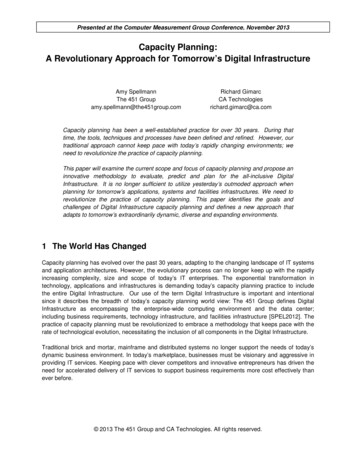
Figure 3: Six weeks (42 days) of incoming traffic (totally 1008 data points; note that two close-to-zero datapoints are invalid)whelms the consumer, the incoming events will be queuedand a non-trivial relay lag will result due to an events queuebacklog. To minimize relay lags, appropriate capacity planning is needed after careful consideration of both producingand consuming rates.2.2 Periodic pattern of incoming traffic rateWe first studied the incoming traffic rate of multiple Espresso instances across many months; our first impression wasthe strong periodic pattern - the traffic shape is repeated foreach day of the week. Figure 3 below shows 42 consecutivedays of data for a single Espresso node. The incoming trafficconsists of two types of database events: insert and update.Databus Relay processes both types of traffic, so we aggregated the total incoming rate for each minute.We observed weekly repeating patterns in incoming traffic rates. Every week, the five workdays have much highertraffic rates than the two weekends. Such a weekly patternrepeats with similar traffic shapes. Within a single day, irrespective of being workday or weekend, we found that thetraffic rate peaks during regular business hours, while dropsto the lowest at night.(a) Monday traffic (May 5th, 2014)2.3 Incoming traffic of individual days(b) Saturday traffic (May 17th, 2014)We then studied the periodic pattern of incoming trafficfor each day. For each workday and weekend, we noticedthat the traffic shape is a well formed curve. In Figure 4,we show the workday of May 5th , 2014 (Monday) and theweekend day of May 17th , 2014 (Saturday).We observed that the traffic shapes of these two days werequite similar, except for the absolute values of each datapoint. Specifically, for each day, the peak periods were about8 hours (that is, 6AM to 2PM in the West Coast, or 9AMto 5PM in the East Coast). Not surprisingly, the workdaypeak value (6367 records/sec) was much higher than that ofweekends (1061 records/sec).Figure 4: Individual days of traffic (Each data pointrepresents 5 minutes, totally 288 data points)A critical performance factor is the Databus Relay Lag(i.e., Databus replication latency), which is calculated asthe difference in time between when a record is insertedinto source Espresso and when the record is ready to beconsumed by the Databus clients. The extent of relay laglargely depends on two factors: the rate of incoming rawdatabase events (i.e., the “producing rate” of the events)and the Databus Relay processing capacity (i.e., the “consuming rate” of the events). So if the producing rate isalways lower than the consuming rate, there will be no substantial relay lags, other than the event transmission delaywhich is usually very small. But when the producer over-2.4 Relay processing capacityWe also examined the relay processing capacity. The relay processing rate was maximized only when there was abuildup in queued events. To force Databus Relay to work at41

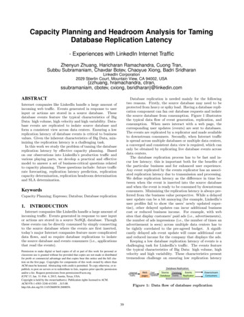
tency can accumulate during peak hours when productionrate is higher than the relay capacity, and the accumulatedreplication latency decreases during non-peak hours whenthe incoming traffic rate is lower than the relay capacity.The incoming traffic rate keeps growing, thanks to theuser and activity growth, so it is important to take intoaccount the traffic growth when doing capacity planning.We need to forecast into future traffic to understand thefuture replication latency, estimate the capacity headroom,define the replication capacity requirements, and determineSLAs.Figure 5: Relay processing rate (Relay capacity)3. PROBLEM DEFINITIONIn this section, we formally define the problems we attempt to address in this work. We first give the definitionsof SLAs (service level agreements); then present the fourtypes problems related to capacity planning.3.1 Forms of SLA (service level agreements)SLA is a part of a service contract where a service is formally defined. Thought normally the service contracts arebetween companies, it can extend to between different divisions inside a company or even between different softwarecomponents. For instance, a web service component may define a SLA such as maximum call latency being 100 ms, sothat the callers (e.g., a web page rendering component) canrely on the SLA to make design choices and further definetheir SLAs.The goal of taming the database replication latency is tofulfill SLA, which can come in different forms. A straightforward SLA metric can be expressed as the “largest” replication latency experienced, which is the form we use to describe our designs. For instance, largest replication latencyshould not exceed 60 seconds.However, other forms ofSLA metrics are also possible, depending on specific requirements. To give a few examples: (1) certain percentiles (e.g.,p99) of all replication latencies in a day, or (2) the durationof replication latencies exceeding certain values. Despite thedifferences in SLA forms, we believe the underlying mechanisms required to answer the five types of questions in Section 1 are very similar. So in this work, we will use thelargest replication latency as the SLA metric to present oursolution.Figure 6: Traffic growth in 6 weeksfull capacity, we rewound the starting System Change Number (SCN) of the relay component to artificially introducesufficient relay lag. For a particular Databus Relay instance,the replay processing rates over 20 hours of a recent day areplotted in Figure 5.We observed that the relay processing rate is relativelyflat over time. The reason for relative stable relay processing rate is because the processing rate is dominated by thereplication protocol, which is relatively constant for eachevent.2.5 Growing trafficWe studied the historical data of incoming traffic andfound that: (1) overall, the traffic volume grows over time;(2) the traffic for individual days is affected by many factorsincluding weekends, holidays, and production releases. Weanalyzed the incoming traffic rates for a duration of 6 weeksand plotted the monthly traffic rates in Figure 6. Linearfitting of the curve demonstrates about 20% increase in 6weeks.Note that this analysis and graph are based on a particular instance of the Espresso node. We also studied other instances and found that though the exact growth rates differfor different periods and instances, the overall traffic growthrate is quite significant. Even though it is possible to buildcapacity planning models for each instance for higher accuracy, we want to build a generic model to cover all instances.3.2 Problems being addressedFor simplicity in presentation, we fix the time-granularityof the traffic rates to per-hour average, but other granularitycan be similarly defined. The following variables are neededto define the problems: (1) Relay capacity: Ri,j in day diand hour hj , where 0 j 23; (2) Incoming traffic rate:Ti,j in day di and hour hj ; (3) Replication latency: Li,j inday di and hour hj ; (4) SLA of replication latency: Lsla ,which is the largest replication latency.With the above variables, we can formally define the setof the problems we will address in this work: Forecast future traffic rate Given the historical trafficrate of Ti,j of time period P (e.g., past 30 days), whatare the future traffic rate Tr,k , where r imax in dayr and hour k?2.6 SummaryOur study of LinkedIn’s production traffic showed thatthe database events producing rate (i.e., the incoming trafficrate) follows strong patterns in the form of repeated weeklycurves, while the consuming rate (i.e., the replication processing capacity) is relatively constant. Because of varyingincoming traffic rates, we used to see that replication la- Determine the replication latency Given the trafficrate of Ti,j and relay capacity Ri,j , what are the replication latency of Li,j ?42

Determine required replication capacity Given SLArequirement Lsla and traffic rate of Ti,j , what are required relay capacity of Ri,j ?of future days using ARIMA model and (2) Step-II of forecasting the average rates per hour of each future days usingseasonal indexes.Regression analysis is targeted for estimating the relationships among variables. Regression analysis can also be usedto forecast and predict. Specifically, for our purpose of forecasting future traffic rate, the independent variable is thetime, while the dependent variable is the traffic rate at eachtime. Such analysis is also referred to as “time series regression”. Since we observed strong seasonal pattern with theperiod of a week, we propose to forecast the average traffic rates of future “weeks” based on historical weekly data.Once we obtained the weekly average, we can then convertthe weekly average to per-hour data of within a week usingthe same step-2 of time series model presented above. Another important reason why we choose per-week aggregationis that, regression analysis is based on the assumption thatthe adjacent data points are not dependent. Compared tofiner scale of data points, weekly aggregated data are lessdependent on each other. We will discuss more on this inSection 7.For answering the other three types of capacity-planningrelated questions, we develop respective mechanisms whichutilize numerical calculations and binary-searching. For easeof description, we assume the time granularity is per-hour.Once the traffic rates are obtained, then a numerical calculation method will be used to deduct the relay lags of anytime point. Based on the numerically calculated results, therelay capacity required to sustain a particular traffic rate canalso be obtained using binary search. The maximum traffic rates as well as the corresponding future dates can alsobe determined. Finally, examining the deducted replicationlatencies we can also determine appropriate SLAs. Determine replication headroom There are two questions: (1) Given the SLA of Lsla and relay capacity ofRi,j , what are the highest traffic rate Ti,j it can handle without exceeding SLA? (2) what are the expecteddate dk of the previous answer? Determine SLA There are multiple forms of SLAs thatcan be determined. In this work we consider two ofthem: (1) what is the largest replication latency Lmaxin a week; (2) for 99% of time in a week the replicationlatency should not exceed Lp99 , what is the Lp99 value?4.DESIGNThis section will start with the overview of our design, followed by two models to perform forecasting of future trafficrates. After that, the other four types of questions describedin Section 1 will be respectively answered.4.1 Design overviewBefore we jump into the details of the design, it helps togain a conceptual grasp of the problem we try to address.The extent of relay lag largely depends on two factors: therate of incoming raw database events and the Databus Relay processing capacity. The Databus Relay is conceptuallya queuing system and has the features of a single server,a First-In-First-Out (FIFO) queue, and infinite buffer size.Unlike typical queuing theory problems, in this work, we aremore focused on the “maximum” awaiting time of all eventsat a particular time.In order to answer all the capacity planning questions, weneed to obtain the future traffic rates. We will employ twomodels for traffic forecasting: Time series model and Regression analysis. Given historical traffic rates of certain period,the time series model will be able to forecast the future ratesbased on the discovered trend pattern and seasonal pattern.The historical data we can obtain is mostly per-hour baseddue to current limitations on the storing mechanisms, so foreach past day it consists of 24 data points. We also observed that the traffic rates exhibit strong seasonal patternwith period of a week (i.e., 7 days, or 168 hours).For this type of time series data, typically ARIMA (autoregressive integrated moving average) model [3] is chosenfor modeling and forecasting. Due to its design rationalesand computation overhead, ARIMA is not suitable for longperiod seasonality (e.g., 168). In addition, the capacity planning needs to obtain per-hour forecasted data rather thanper-day data. Because of this, we are not allowed to aggregate per-hour data into per-day data to reduce seasonalityperiod to 7 (since a week has 7 days). To accommodatethe long period seasonality as observed in traffic data andthe per-hour forecasting requirements, we propose a twostep forecasting model to obtain future per-hour traffic rates.Briefly, it firstly obtain the aggregated traffic volume of eachday/week, it then “distribute” (or “convert”) the aggregateto each hour inside a day/week. The “conversion” of trafficvolume from day/week to hours relies on seasonal indexes,which roughly represent the traffic portion of each hour inside a week. Specifically, the model consists of two steps:(1) Step-I of forecasting the average incoming rates per day4.2 Forecasting future traffic rate with ARIMA modelThe incoming traffic rates of each time unit are a sequenceof observations at successive points in time, hence they canbe treated as a time series. We can employ time seriesmethod to discover a pattern and extrapolate the patterninto the future. The discovered pattern of the data can helpus understand how the values behave in the past; and theextrapolated pattern can guide us to forecast future values.ARIMA time series forecasting model will be used to predict the incoming rates of any future days. Though it isobvious to see the weekly pattern for our particular time series data, identifying seasonal periods for other time seriesmight not be so trivial. Examining the ACF (Autocorrelation Function) [3], we see a strong signal at 7, indicatinga period of 1 week (i.e., 7 days). Based on our investigations into the properties of the traffic data, we decided touse ARIMA(7,1,0) to fit the historical data and forecast thetraffic rates of future days, the details will be presented inSection 5.Answering various capacity planning questions requiresthe per-hour granularity of traffic rates. To convert the forecasted per-day rate to per-hour rate, we perform time seriesdecomposition. A typical time series consists of three components: trend component, cycle (or seasonal) componentand irregular component [3]: Xt Tt St Rt , where: Xtis the value of the series at time t; Tt is the trend component,St is the seasonal component, and Rt is the random effector irregular component. Tt exists when the time series data43

Li,j predict(Ti,j , Ri,j ): // Latency in seconds.12345678Ri,j capacity(Ti,j , Lsla ):// assuming no latency buildup in di 1 , so Li,0 0.for each hour of hj , where 1 j 24:if Ti,j Ri,j : // increase latency buildup3600(Ti,j Ri,j )Li,j Li,j 1 Ri,jelse: //decrease latency buildup if any3600(Ri,j Ti,j )Li,j Li,j 1 Ri,jif Li,j 0:Li,j 0variables:1 Ri,j(min) : a Ri,j such that max(Li,j ) Lsla2 Ri,j(max) : a Ri,j such that max(Li,j ) Lsla12345678910Figure 7: Algorithm of predicting replication latencygradually shift across time; St represents repeating patterns(e.g., daily or weekly); while Rt is time-independent and ischaracterised by two properties: (1) the process that generates the data has a constant mean; and (2) the variabilityof the values is constant over time.Time series decomposition can eliminate the seasonal component based on seasonal index, which measures how muchthe average for a particular period tends to be above (orbelow) the expected value. Seasonal index is an averagethat can be used to compare an actual observation relativeto what it would be if there were no seasonal variation. Inthis work, we utilize seasonal index to convert per-day datato per-hour data. Calculating seasonal index requires thesetting of seasonal period, which we choose 168 hours (i.e.,1week, or 7 days * 24 hours). Once the seasonal indexes arecalculated, each day of data can be “seasonalized” to obtainper-hour data based on the particular day in a week. Wewill present details in Section 5.Ri,j(lf ) Ri,j(min)Ri,j(rt) Ri,j(max)while Ri,j(lf ) Ri,j(rt) 1:R RRi,j(mid) i,j(lf ) 2 i,j(rt)Li,j predict(Ti,j , Ri,j(mid) )if max(Li,j ) Lsla :Ri,j(rt) Ri,j(mid)else:Ri,j(lf ) Ri,j(mid)return Ri,j(rt)Figure 8: Algorithm of determining replication capacitywill be consumed by the end of non-peak traffic time of anyday. This is a reasonable assumption as otherwise the replication latency will continually grow across days, which isunusable scenario for any business logic or SLA definition.The mechanism to predict replication latency for any hourof a day is based on numerical calculations. Assuming thereis no latency buildup from previous day of di 1 (i.e., Li,0 0, for each successive hour hj where j 0, the traffic rateis compared to relay capacity at hj . If the incoming rateis higher, it will incur additional replication latency at thattime. Otherwise, previous replication latency, if any, will bedecreased, as the relay has additional capacity to consumepreviously built-up latency. The amount of latency change isbased on the difference between the two rates, that is, Lδ Ti,j Ri,jhours. This process continues for each hour thatRi,jfollows, and the entire data set of relay lag is constructed.The algorithm is shown in Figure 7.4.3 Forecasting future traffic rate with regression analysisWhen regression analysis (i.e., time series regression) isused to forecast future traffic rates, the weekly average values are used instead. Specifically, for the consecutive weeklyaverage traffic rate of Wt , where t is the week id, a trendline (i.e., the linear fitting of Wt ) can be obtained in theform of Yt aWt b. The a is the slope of the change, orthe growth rate. With the trend line, future weekly averagetraffic rate Wt can be forecasted.Future Wt values obtained with time series regression areactually the “deseasonalized” forecast values. To convert tospecific hourly rate, Wt needs to be “seasonalized”, similarto the process of using ARIMA model. The details of theconversion will be presented in Section 5.4.5 Determining replication capacityGiven SLA requirement Lsla (i.e., the maximum allowedreplication latency) and traffic rate of Ti,j , we need to obtainthe minimum required relay capacity of Ri,j . Previously wehave shown how to predict the replication latency Li,j givenTi,j and Ri,j . For simplicity we denote the process as afunction of predict(), so we have Li,j predict(Ti,j , Ri,j ).For each day di , we can also easily obtain the maximumreplication latency of Li,max of Li,j , denoted by Li,max max(Li,j ).To find out the relay capacity Ri,j that having Li,max Lsla , we can do a binary searching on the minimum value ofRi,j . In order to do binary searching, we

Database replication latency is closely tied to capacity planning. Capacity planning will help understand the cur-rent business and operational environment, assess and plan for future application needs based on traffic forecasts. Ca-pacity planning can particularly help reduce the business operation cost. For example, given incoming traffic .