WIXLIB

The Pairwise Multiple Comparison of MeanRanks Package (PMCMR)Thorsten Pohlertlatest revision: 2015-11-19 Thorsten Pohlert. This work is licensed under a Creative Commons License (CC BY-ND4.0). See http://creativecommons.org/licenses/by-nd/4.0/ for details. Please cite thispackage as:T. Pohlert (2014). The Pairwise Multiple Comparison of Mean Ranks Package (PMCMR). Rpackage. http://CRAN.R-project.org/package PMCMR.See also citation("PMCMR").Contents1 Introduction22 Comparison of multiple independent samples (One-factorial design)2.1 Kruskal and Wallis test . . . . . . . . . . . . . . . . . . . . . . . . . .2.2 Kruskal-Wallis – post-hoc tests after Nemenyi . . . . . . . . . . . . . .2.3 Examples using posthoc.kruskal.nemenyi.test . . . . . . . . . . .2.4 Kruskal-Wallis – post-hoc test after Dunn . . . . . . . . . . . . . . . .2.5 Example using posthoc.kruskal.dunn.test . . . . . . . . . . . . . .2.6 Kruskal-Wallis – post-hoc test after Conover . . . . . . . . . . . . . . .2.7 Example using posthoc.kruskal.conover.test . . . . . . . . . . . .2.8 Dunn’s multiple comparison test with one control . . . . . . . . . . . .2.9 Example using dunn.test.control . . . . . . . . . . . . . . . . . . .2.10 van der Waerden test . . . . . . . . . . . . . . . . . . . . . . . . . . . .2.11 Example using vanWaerden.test . . . . . . . . . . . . . . . . . . . . .2.12 post-hoc test after van der Waerden for multiple pairwise comparisons2.13 Example using posthoc.vanWaerden.test . . . . . . . . . . . . . . .223467891010111212123 Comparison of multiple joint samples (Two-factorial unreplicated completeblock design)133.1 Friedman test . . . . . . . . . . . . . . . . . . . . . . . . . . . . . . . . . . 131

3.23.33.43.5Friedman – post-hoc test after Nemenyi . . . . . .Example using posthoc.friedman.nemenyi.testFriedman – post-hoc test after Conover . . . . . .Example using posthoc.friedman.conover.test.131416161 IntroductionFor one-factorial designs with samples that do not meet the assumptions for one-wayANOVA (i.e., i) errors are normally distributed, ii) equal variances among the groups,and, iii) uncorrelated errors) and subsequent post-hoc tests, the Kruskal-Wallis test(kruskal.test) can be employed that is also referred to as the Kruskal–Wallis one-wayanalysis of variance by ranks. Provided that significant differences were detected by theKruskal-Wallis-Test, one may be interested in applying post-hoc tests for pairwise multiple comparisons of the ranked data (Nemenyi’s test, Dunn’s test, Conover’s test). Similarly, one-way ANOVA with repeated measures that is also referred to as ANOVA withunreplicated block design can also be conducted via the Friedman test (friedman.test).The consequent post-hoc pairwise multiple comparison tests according to Nemenyi andConover are also provided in this package.2 Comparison of multiple independent samples (One-factorialdesign)2.1 Kruskal and Wallis testThe linear model of a one-way layout can be written as:yi µ αi i ,(1)with y the response vector, µ the global mean of the data, αi the difference to the meanof the i-th group and the residual error. The non-parametric alternative is the Kruskaland Wallis test. It tests the null hypothesis, that each of the k samples belong to thesame population (H0 : R̄i. (n 1)/2). First, the response vector y is transformed intoranks with increasing order. In the presence of sequences with equal values (i.e. ties),mean ranks are designated to the corresponding realizations. Then, the test statistic canbe calculated according to Eq. 2:12Ĥ n (n 1) "Xki 1#Ri2 3 (n 1)ni(2)with n ki ni the total sample size, ni the number of data of the i-th group and Ri2the squared rank sum of the i-th group. In the presence of many ties, the test statisticsĤ can be corrected using Eqs. 3 and 4PPi rC 1 3i 1 ti tin3 n2 ,(3)

with ti the number of ties of the i-th group of ties.Ĥ Ĥ/C(4)The Kruskal and Wallis test can be employed as a global test. As the test statisticH̄ is approximately χ2 -distributed, the null hypothesis is withdrawn, if Ĥ χ2k 1;α .It should be noted, that the tie correction has only a small impact on the calculatedstatistic and its consequent estimation of levels of significance.2.2 Kruskal-Wallis – post-hoc tests after NemenyiProvided, that the globally conducted Kruskal-Wallis test indicates significance (i.e.H0 is rejected, and HA : ’at least on of the k samples does not belong to the samepopulation’ is accepted), one may be interested in identifying which group or groupsare significantly different. The number of pairwise contrasts or subsequent tests thatneed to be conducted is m k (k 1) /2 to detect the differences between each group.Nemenyi proposed a test that originally based on rank sums and the application of thefamily-wise error method to control Type I error inflation, if multiple comparisons aredone. The Tukey and Kramer approach uses mean rank sums and can be employed forequally as well as unequally sized samples without ties (Sachs, 1997, p. 397). The nullhypothesis H0 : R̄i R̄j is rejected, if a critical absolute difference of mean rank sumsis exceeded.v#u "q ;k;α un(n 1)11R̄i R̄j t ,122ninj(5)where q ;k;α denotes the upper quantile of the studentized range distribution. Although these quantiles can not be computed analytically, as df , a good approximation is to set df very large: such as q1000000;k;α q ;k;α . This inequality (5) leadsto the same critical differences of rank sums ( Ri Rj ) when multiplied with n forα [0.1, 0.5, 0.01], as reported in the tables of Wilcoxon and Wilcox (1964, pp. 29–31).In the presence of ties the approach presented by Sachs (1997, p. 395) can be employed(6), provided that (ni , nj , . . . , nk 6) and k 4.:v#u "un(n 1)11R̄i R̄j tCχ2k 1;α ,12ninj(6)where C is given by Eq. 3. The function posthoc.kruskal.nemenyi.test does notevaluate the critical differences as given by Eqs. 5 and 6, but calculates the correspondinglevel of significance for the estimated statistics q and χ2 , respectively.In the special case, that several treatments shall only be tested against one controlexperiment, the number of tests reduces to m k 1. This case is given in section 2.8.3

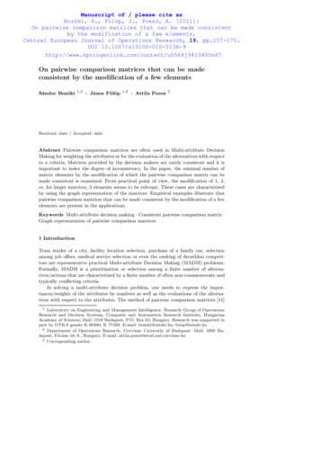
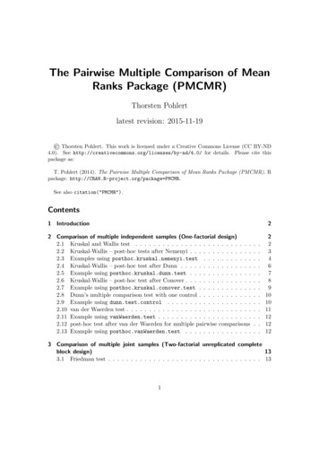
2.3 Examples using posthoc.kruskal.nemenyi.test152025The function kruskal.test is provided with the library stats (R Core Team, 2013).The data-set InsectSprays was derived from a one factorial experimental design andcan be used for demonstration purposes. Prior to the test, a visualization of the data(Fig 1) might be helpful:10 05 ABCDEFFigure 1: Boxplot of the InsectSprays data set.Based on a visual inspection, one can assume that the insecticides A, B, F differ fromC, D, E. The global test can be conducted in this way: kruskal.test(count spray, data InsectSprays)Kruskal-Wallis rank sum testdata: count by sprayKruskal-Wallis chi-squared 54.6913, df 5, p-value 1.511e-104

As the Kruskal-Wallis Test statistics is highly significant (χ2 (5) 54.69, p 0.01),the null hypothesis is rejected. Thus, it is meaningful to apply post-hoc tests with thefunction posthoc.kruskal.nemenyi.test. s)posthoc.kruskal.nemenyi.test(x count, g spray, dist "Tukey")Pairwise comparisons using Tukey and Kramer (Nemenyi) testwith Tukey-Dist approximation for independent samplesdata:BCDEFcount and 0.00585E0.00031P value adjustment method: noneThe test returns the lower triangle of the matrix that contains the p-values of thepairwise comparisons. Thus R̄A R̄B : n.s., but R̄A R̄C : p 0.01. Since PMCMR1.1 there is a formula method included. Thus the test can also be conducted in thefollowing way: posthoc.kruskal.nemenyi.test(count spray, data InsectSprays, dist "Tukey")Pairwise comparisons using Tukey and Kramer (Nemenyi) testwith Tukey-Dist approximation for independent samplesdata:BCDEFcount by 0.00585E0.00031P value adjustment method: noneAs there are ties present in the data, one may also conduct the Chi-square approach:5

(out - posthoc.kruskal.nemenyi.test(x count, g spray, dist "Chisquare"))Pairwise comparisons using Nemenyi-test with Chi-squaredapproximation for independent samplesdata:BCDEFcount and 0.02955E0.00281P value adjustment method: nonewhich leads to different levels of significance, but to the same test decision. Thearguments of the returned object of class pairwise.h.test can be further explored.The statistics, in this case the χ2 estimations, can be taken in this way: print(out statistic)BCDEFABCDE0.09741248NANANANA22.70093702 25.772474315NANANA9.68046043 11.720034247 2.7330908NANA14.76750381 17.263698630 0.8495291 0.5351027NA0.16383657 0.008585426 26.7218417 12.3630375 18.04226The test results can be aligned into a summary table as it is common in scientificarticles. However, there is not yet a function included in the package PMCMR. Therefore,Table 1 was manually created.2.4 Kruskal-Wallis – post-hoc test after DunnDunn (1964) has proposed a test for multiple comparisons of rank sums based on the zstatistics of the standard normal distribution. The null hypothesis (H0), the probabilityof observing a randomly selected value from the first group that is larger than a randomlyselected value from the second group equals one half, is rejected, if a critical absolutedifference of mean rank sums is exceeded:v#u "u n (n 1)11R̄i R̄j z1 α/2 t B ,126ninj(7)

with z1 α/2 the value of the standard normal distribution for a given adjusted α/2 level depending on the number of tests conducted and B the correction term for ties,which was taken from Glantz (2012) and is given by Eq. 8:Pi rB t3i ti12 (n 1)i 1 (8)The function posthoc.kruskal.dunn.test does not evaluate the critical differencesas given by Eqs. 7, but calculates the corresponding level of significance for the estimatedstatistics z, as adjusted by any method implemented in p.adjust to account for TypeI error inflation. It should be noted that Dunn (1964) originally used a Bonferroniadjustment of p-values. For this specific case, the test ist sometimes referred as to theBonferroni-Dunn test.2.5 Example using posthoc.kruskal.dunn.testWe can go back to the example with InsectSprays. s)posthoc.kruskal.dunn.test(x count, g spray, p.adjust.method "none")Pairwise comparisons using Dunn's-test for multiplecomparisons of independent samplesdata:count and sprayABCB 0.75448 C 1.8e-06 3.6e-07 D 0.00182 0.00060 0.09762D-E-Table 1: Mean rank sums of insect counts (R̄i ) after the application of insecticides(Group). Different letters indicate significant differences (p 0.05) according to the Tukey-Kramer-Nemenyi post-hoc test. The global test according toKruskal and Wallis indicated significance (χ2 (5) 54.69, p 0.01).GroupR̄iC11.46 aE19.33 aD25.58 aA52.17 bB54.83 bF55.62 b7

E 0.00012 3.1e-05 0.35572 0.46358 F 0.68505 0.92603 2.2e-07 0.00043 2.1e-05P value adjustment method: noneThe test returns the lower triangle of the matrix that contains the p-values of thepairwise comparisons. As p.adjust.method "none", the p-values are not adjusted.Hence, there is a Type I error inflation that leads to a false postive discovery rate. Thiscan be solved by applying e.g. a Bonferroni-type adjustment of p-values. s)posthoc.kruskal.dunn.test(x count, g spray, p.adjust.method "bonferroni")Pairwise comparisons using Dunn's-test for multiplecomparisons of independent samplesdata:BCDEFcount and 0.00640E0.00031P value adjustment method: bonferroni2.6 Kruskal-Wallis – post-hoc test after ConoverConover and Iman (1979) proposed a test that aims at having a higher test power thanthe tests given by inequalities 5 and 6:v "#"#u un 1 Ĥ11R̄i R̄j t1 α/2;n k ts2 ,n kninj(9)with Ĥ the tie corrected Kruskal-Wallis statistic according to Eq. 4 and t1 α/2;n kthe t-value of the student-t-distribution. The variance s2 is given in case of ties by:X(n 1)21s Ri2 nn 14"2#(10)The variance s2 simplifies to n (n 1) /12, if there are no ties present. AlthoughConover and Iman (1979) did not propose an adjustment of p-values, the function8