WIXLIB

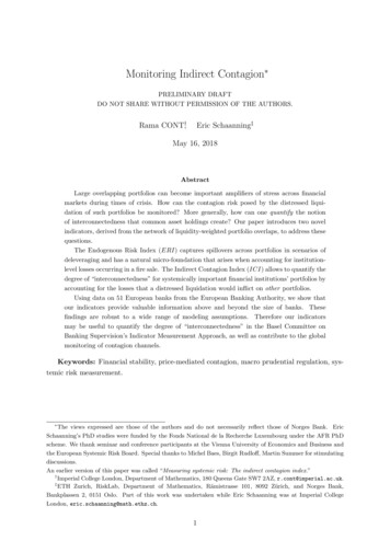
Main contributions.1. Endogenous Risk Index: Given portfolio holdings data, we construct a network ofindirect contagion which is based on the overlap of institutions’ portfolios, adjusted forthe liquidity of the underlying assets. We introduce the Endogenous Risk Index (ERI),the Perron-eigenvector of this liquidity-weighted overlap matrix of portfolios, and showthat it has a natural micro-foundation that comes from correctly quantifying mark tomarket losses in deleveraging scenarios. The ERI is shown to be a good proxy of spilloverlosses over and above the size of portfolios. In particular, accounting for the liquidity ofthe underlying assets in the portfolio improves the prediction of fire sales losses markedly.The ERI can function as a proxy for monitoring contagion in periods between stress tests.2. Indirect Contagion Index: The Indirect Contagion Index (ICI) is a modified versionof the Endogenous Risk Index, which ignores self-inflicted liquidation losses and stresseslosses caused to other portfolios. In the framework of the Basel Committee on BankingSupervision’s GSIB methodology the ICI could be used as an additional indicator toquantify the degree of interconnectedness of systemically important institutions. Usingdata from the 2016 EBA stress test, we find that relating to the price-mediated contagionchannel, Crédit Agricole, Deutsche Bank, BNP Paribas, Société Générale and Barclays areamong the most systemic institutions.The predictive power of our indicators is robust to a wide range of modeling assumptions suchas the liquidation strategies which institutions use to delever portfolios, or the scenarios thattrigger these.Structure.The paper is organised as follows: Section 2.1 is devoted introduces our frameworkto monitor indirect contagion. Section 2.2 and 2.3 present the Endogenous Risk Index and theIndirect Contagion Index respectively. Sections 3.1 and 3.2 apply our methodology to a datasetof European Banks. Moreover, we perform a large sensitivity analysis in Section 3.3. andintroduce an optimal bank response in Section 3.4. Section 3.5 compares the ERI and ICI toother measures of overlap, while Section 3.6 suggests an application of the indicators to monitorGlobal Systemically Important Banks (GSIBs) in the Basel Committe on Banking Supervisions’framework. Section 4 concludes.22.1Monitoring indirect contagionFire-sales losses and liquidity-weighted overlapsWe consider a financial network consisting of i 1.N institutions and µ 1.M securities. Theinstitutions are subject to regulatory, market- or self-imposed constraints, which may dependon their capital, leverage or liquidity levels. Let Πi,µ denote the value of institution i’s holdingsin asset class µ in monetary units. The portfolio holdings of the entire system are given by thematrix Π RN M . This matrix corresponds to a bi-partite network of institutions and assetclasses, as shown in Figure 1.5

Figure 1: Bipartite network of institutions A-K and asset classes 1-4, which gives rise to anetwork of indirect contagion between institutions.Such a network can give rise to indirect contagion: Even though institutions A through Emay have no connection, institutions B to E may suffer losses if for some reason A is forced toliquidate its position in asset class 1, thereby depressing its price. Specifically, two types of lossescan arise: (i) mark-to-market losses on remaining holdings, suffered by all parties that hold theasset undergoing the distressed liquidation and (ii) implementation costs which the liquidatinginstitution suffers on the position it is trying to liquidate. Moreover, if, as a result of the forceddeleveraging by A, institutions B or D need to liquidate a part of their portfolio, the price ofasset class 2 may drop and cause losses for institutions F and G, who were previously unaffected.This shows how overlapping portfolios can become a driver of cross-asset class contagion, evenwhen the asset classes are economically and geographically essentially independent.In order to quantify this phenomenon properly, we need to specify: (i) when institutions react toa shock, (i) how they react when forced to, and (iii) how prices respond to forced liquidations.Using these three building blocks, we show that an endogenous risk index naturally arises whenone quantifies the liquidation losses in such a network of constrained and overlapping portfolios.The presentation follows the model discussion in Cont and Schaanning (2016), to which werefer the reader for further details:1. At time k 1, in response to a stress scenario, parametrised by percentage shocks to assetclasses [0, 1]M , some institutions j deleverage their portfolio by selling a proportionΓjk ( ) [0, 1] of marketable assets. In Section 3.4, we assume that banks do not sell assetsproportionately, but choose Γj so as to minimise the liquidation losses they suffer. ThisPj,µ jleads to an aggregate amount qkµ Nj 1 Πk 1 Γk ( ) of sales in asset class µ. In general, thedeleveraging proportion, Γjk ( ) can depend on the capital buffer, the liquidity reserves andother balance sheet components of institution j. In particular, when j is well-capitalisedand has a prudent liquidity buffer, it will be able to withstand the shock without resortingto distressed liquidations, in which case Γj ( ) 0. We specify Γ precisely in the empirical6

section and will drop the in Γ( ) for notational convenience.2. The market price of asset class µ is denoted by Skµ . The impact of asset sales results in adecline of the market price, moving it toSkµwhere the market depth Dµ (τ ) µSk 1 qkµ,1 DµADVµ τσµ(1)is proportional to the ratio of the averagedaily volume (ADV) and the volatility of the asset class times the liquidation horizon, τ ,which is assumed to be τ 20 days in our calibration. This corresponds to a linear priceimpact function SS Ψµ (x) : xDµ ,as used in ((Obizhaeva, 2012), (Kyle and Obizhaeva,2016), (Amihud, 2002), (Cont and Wagalath, 2016)). For a more general discussion onnon-linear price impact functions in the context of stress testing, we refer to (Cont andSchaanning, 2016).3. For any institution i, the combined effect of its own deleveraging (if it occurs) and theimpact of other forced sales changes the market value of its holdings in asset class µ toPrevious valueΠi,µk z } {Πi,µk 1 1 Γik {z } 1 Dµ 1NX .Γjk Πj,µk 1(2)j 1Remainder after deleveraging by i {z}Price impact on remaining holdingsImportantly, this shows that in general the value of institution i’s holdings under stresscannot be simply inferred from historically observed returns and covariances, but maydepend on the stress scenario and the network of overlapping portfolios.The price move generates two types of losses for portfolio i: First, it causes mark to marketlosses on the remaining part of the portfolio given byMki M X i,µ (1 Γik )(1 Γik )Πi,µk 1 ΠkΠi,µk 1 NXDµ 1 Γj Πj,µ kµ 1µ 1 (1 Γik )MXj,µN XMXΠi,µk 1 Πk 1Dµj 1 µ 1k 1j 1Γjk .(3)A second source of loss stems from the fact that assets are not liquidated at the current marketprice but at a discount. We assume for simplicity that the deleveraging institutions suffer thesame price impact on the liquidated part of the portfolio as on their remaining part, yieldingthe realised lossRki M XΓik Πi,µk 1 Γik Πi,µk 1 µ 1 Γikj,µN XMXΠi,µk 1 Πk 1j 1 µ 1Dµ7Γjk .qkµ1 Dµ (4)

Summing (4) and (3) yields the total loss of portfolio i at the k-th round of deleveraging:Lik j,µN XMXΠi,µk 1 Πk 1Dµ{zj 1 µ 1 Γjk NXjΩijk 1 Γk ,j 1Ωij (Πk 1 )}which shows that the magnitude of fire sales spillovers from institution i to institution j isproportional to the liquidity-weighted overlap Ωij between portfolios i and j (Cont and Wagalath,2013):Ωij (Πk ) : MXΠi,µ Πj,µkµ 1kDµ.Let D : diag(D1 , . . . , DM ), then the matrix of portfolio overlapsΩ(Πk ) Πk D 1 Π k,(5)can be viewed as a (liquidity-)weighted adjacency matrix of the network linking portfoliosthrough their common holdings.2.2The Endogenous Risk Index.From the derivation above, it follows that in the first round, the fire-sales losses for all banksare given by the vectorF Loss ΩΓ.(6)As Ω is symmetric positive semi-definite by construction, we know that there exists an orthonormal basis of eigenvectors with real eigenvalues for it. We further assume that Ω is anirreducible and non-negative matrix. This is equivalent to the network of overlapping portfoliosbeing strongly connected (i.e. it is not a union of disjoint sub-networks) and that there are noPΠi,µ Πj,µpairs of portfolios such that M 0 respectively. The European banking networkµ 1Dµwhich we use in our empirical analysis verifies these assumptions. Under these conditions, thePerron-Frobenius theorem ensures that the components of the first eigenvector are all positive.If the first eigenvalue dominates, the network of liquidity-weighted portfolio overlaps can beapproximated well by a one-factor modelΩ λ1 uu ,(7)where u is the Perron eigenvector corresponding to the largest eigenvalue λ1 . Using this approximation, the fire-sales loss can be written asiF Loss λ1 uiNXj 18uj Γj ( ).

Taking logarithms, we getlog(F Lossi ) log(λ1 uiNXuj Γj ( ))j 1 {z}1 log(ui ) log(λ1 ) log(u Γ( )), {z}slope(8)Interceptwhich implies that the logarithm of the Perron eigenvector should be a good predictor of fire-saleslosses. Moreover, we should expect a slope of approximately one when regressing log-fire-saleslosses on it.Equation (8) motivates the introduction of the following definition: The Endogenous RiskIndex (ERI) of a financial institution is its component i in the Perron eigenvector ui of thematrix Ω from (5) of liquidity-weighted portfolio overlaps:ERI(i) ui .(9)The EIR provides a measure of centrality of the node i in the network whose links are weightedby the overlap matrix Ω. The ERI is constructed as follows:1. Collect portfolio holdings Πi,µ by asset class for each financial institution in the network,at the granularity level corresponding to bank stress tests.2. Estimate a market depth parameter Dµ ADVµσµfor each asset class.3. Check that Ωij 0 and that Ω is irreducible.4. Compute the largest eigenvalue and the corresponding eigenvector (the “Perron eigenvector”) u (ui , i 1.N ) of the matrix of liquidity-weighted overlaps Ω(Π) ΠD 1 Π .5. The Endogenous Risk Index is the Perron eigenvector, ERI u.2.3The Indirect Contagion IndexBefore turning to the empirical application, we propose a modification relative to the ERI thatdiscounts the fire-sales losses that a distressed portfolio liquidation would inflict on itself, andonly take into consideration the spillover-losses that are generated to other portfolios. We callthis measure the Indirect Contagion Index (ICI), and compute it as follows:1. Compute Ω ΠD 1 Π , as detailed for the ERI above.2. Compute the largest eigenvalue and the corresponding Perron eigenvector v ofΩ0 : Ω diag(Ω11 , . . . , ΩN N ).23. The Indirect Contagion Index is the Perron eigenvector, ICI v.2Note that the zero diagonal of Ω0 does not make the matrix reducible or violate the non-negativity constraint,and hence the Perron-Frobenius Theorem is still applicable.9

We illustrate the difference between the ERI and the ICI, in a simple financial network of 7banks and 2 asset classes given by:1000Π 10000000! 01100 100 100 100 100 100D (1000, 2000) .Banks 1 and 2 are thus large (and equal in size), while banks 3 - 7 are smaller. Asset class 1 istwice as illiquid as asset class 2. The left panel of Figure 2 shows the network, where the bluesquares denote banks, the red circles denote asset classes and the size of the edge denotes themagnitude of the holding (not to scale). The bigger banks are denoted by larger squares; themore illiquid asset class is depicted by a larger circle. The right panel of Figure 2 shows the ICI(blue bars) and the ERI (black crosses) for this network. Bank 1 clearly dominates the ERIranking. This is due to its main holdings being less liquid compared to Bank 2’s holdings, andthe amount of self-contagion that this could trigger. In contrast, Bank 2 has a large positionin asset class 2, which all the medium-sized banks hold as well. Consequently, even though thesame liquidation volume for Bank 2 in asset class 2 would cause a smaller loss than it wouldfor Bank 1 in asset class 1, if Bank 2 delevers, the rest of the system also suffers significantfire-sales losses. The ICI discounts the self-inflicted fire-sales loss and only accounts for systemexternalities, which is why in the ICI ranking, Bank 2 dominates, and Bank 1 is equally ranked1.0as the medium-sized banks.ICIERIB0.60.40.00.2ERI and ICI0.8A12345671234567BankFigure 2: Illustrative example showing how the ICI discounts self-inflicted losses compared tothe losses caused for other participants relative to the ERI.We will further discuss the difference between the ERI and the ICI for European banks inthe sections below.10

3Empirical Application3.1DataWe use data from the 2016 stress test exercise by the European Banking Authority (EBA)which provides information on notional exposures of 51 European banks across several hundredasset classes.3 Holdings are disaggregated by asset type and geographical region. We subdividemarketable assets into corporate and sovereign bonds, which may be liquidated in a stressscenario. All other asset classes are classified as illiquid assets and assumed to be unavailablefor short-term liquidations (non-securitised exposures). Ignoring asset classes to which theEuropean banking system, as a whole, has an exposure below 1M EUR, leaves us with 93 assetclasses, yielding a 51 93 matrix of liquid holdings Π. The most important regions for corporateexposures, covering over 75% of the total, are France (21.0%), U.S. (14.1%), Germany (11.7%),Italy (6.5%), Spain (4.6%), Netherlands (4.4%) and Belgium (3.2%). The most importantregions for sovereign exposures, covering more than 75% of the total, are Germany (13.8 %),France (13.3%), U.S. (12.8%), Italy (9.2%), U.K. (8.4%), Spain (6.3%), Netherlands (4.6%),Belgium (4.2 %) and Japan (3.4%). Through a similar procedure, we obtain a 51 98 matrix ofilliquid holdings, which we denote Θ. This corresponds to 97 asset classes for commercial andresidential mortgage exposures respectively in the various regions and a 98th entry consisting ofall remaining illiquid asset holdings (intangible goods, defaulted exposures etc).Collectively, the 51 banks hold assets totalling 26.3 trillion EUR, of which 54.6 % (14.3 tnEUR) are in loans and advances, 31.1 % (8.2 tn EUR) are in marketable assets, and 14.3 % (3.8tn EUR) are in “residual” assets classes that are not of relevance for our model.The market depth parameter Dµ defined in (1) is computed following the methodology in(Obizhaeva, 2012) and (Cont and Schaanning, 2016). The estimation procedure is explained inmore detail in Section 3.3, where we perform a sensitivity analysis on this parameter.Empirical analysis.As the portfolio holdings from the 2016 EBA data fulfil all our assump-tions, we compute Ω as well as the ERI and ICI as detailed above. The left-hand panel ofFigure 3 shows that the distribution of liquidity-weighted overlaps Ωij displays considerable heterogeneity. The right panel shows the first twenty ranked eigenvalues of Ω. The first eigenvalueaccounts for about 65% of the total variation and clearly dominates the remaining ones, we thusexpect the ERI to be a good predictor of fire-sales losses in the sequel.Figure 4 shows the Endogenous Risk Index for the European Banking network in 2016, wherewe have labelled the banks with the highest ERI: Crédit Agricole, BNP Paribas, Deutsche Bank,Société Générale and Barclays. All banks that are identified are either Global SystemicallyImportant Banks (GSIBs) or Domestic Systemically Important Banks (DSIB). It is importantto note that the banks are ranked by the amount of contagion they could trigger should theyengage in distressed liquidations. This is not the same as ranking them according to their size– an issue we illustrate in detail in the next section.Finally, Figure 5 depicts the indirect contagion network between European banks as impliedby the EBA data. For visual purposes, we have placed the banks identified as the most systemic3Cont and Schaanning (2016) uses the same data and follow their presentation here.11

605040301020% of variation12864002Percent0 10 1021031041051061071081091010101110125Liquidity weighted overlap (EUR)101520Ranked eigenvaluesFigure 3: Distribution of liquidity-weighted overlaps (left) and the ranked eigenvalues of theindirect contagion rclays01020304050BankFigure 4: The Endogenous Risk Index for the European Banking system. (Data: EBA. Calculations: Authors).by the ERI in the centre, and coloured edges orange that connect these banks with each otheras well as with other banks.3.2Quantifying fire-sales losses with the Endogenous Risk Index.Using the official loss rates of the EBA stress test as starting point, we estimate deleveragingthat may occur as a result and the spillover losses that this may cause. Figure 6 shows theEBA scenario losses for the individual banks in percent of their capital. The 10 most severelyhit banks are Banca Monte dei Paschi di Siena (MdPdS), Allied Irish Banks (AIB), Commerzbank (Com), The Royal Bank of Scotland (RBS), Bayerische Landesbank (BL), RaiffeisenLandesbanken-Holding (RLH), Banco Popular Español (BPE), The Governor and Companyof the Bank of Ireland (GCBI), Cooperatieve Centrale Raiffeisen-Boerenleenbank (CCRB)andLandesbank Baden-Württemberg (LBBW). As the EBA dataset does not provide information12

Figure 5: The EU indirect contagion network.on the liquidity, or the risk weights of individual assets on the balance sheet, we focus on aleverage constraint only. Using supervisory data from the Bank of England, Coen et al. (2017)Loss in EBA scenario in % of Bank's equityshow how the model can be adapted to include risk-weighted capital and liquidity constraints.PKPi,κiii,µ The initial leverage of bank i is λi ( Mκ 1 Θ )/C , where C is the capital ofµ 1 ROtherAIBRBSBPEGCBI CCRB05ComBLRLHLBBW01020304050BankFigure 6: The losses in percent of bank equity that are estimated in the 2016 EBA adversescenario.bank i. After a loss li the leverage increases toPMiλ (Π, Θ, C, l) µ 1 Πi,µ PKi,κκ 1 Θ(C i li ) li.(10)If as a result of the shock the leverage λi exceeds the regulatory constraint λmax 33, then thebank will liquidate a portion, Γi [0, 1], of its marketable assets in order to become compliant13

again with the leverage constraint. The bank thus solves(1 Γi )PMPKi,µ i,κµ 1 Πκ 1 Θ(C i li ) li λb ,for Γi , where λb λmax is a buffer leverage. This yieldsPMiΓ (Π, C, Θ, l) µ 1 Πi,µ PKi,κ κ 1 ΘPMi,µµ 1 Πλb (C i li )! 1 1λi (Π,Θ,C,l) λmax .(11)In Section 3.4, banks will not simply sell assets proportionally but choose assets so as to minimisethe liquidation losses they suffer. On t

Their study shows that insurance com-panies with a higher measure of commonality tend to engage in larger common sales, regardless of portfolio size. We will compare our measures of indirect contagion in detail to cosine similar-ity, and other overlap measures. (Blei and Bakhodir, 2014) use clustering tools from machine