Transcription
Geometryinarchitecture and buildingHans SterkFaculteit Wiskunde en InformaticaTechnische Universiteit Eindhoven
iiLecture notes for ‘2DB60 Meetkunde voor Bouwkunde’The picture on the cover was kindly provided by W. Huisman, Department of Architectureand Building. The picture shows the Olympic Stadium for the 1972 Olympic Games inMunich, Germany, designed by Frei Otto.c 2005–2008 Faculteit Wiskunde en Informatica, TU/e; Hans Sterk
Contents1 Shapes in architecture1.1 A brief tour of shapes . .1.2 Different perspectives . .1.3 Numbers in architecture:1.4 Exercises . . . . . . . . .11911162 3–Space: lines and planes2.1 3–space and vectors . . . . . . . . . . . . . . . . . . . . . .2.2 Describing lines and planes . . . . . . . . . . . . . . . . . .2.3 The relative position of lines and planes: intersections . . .2.4 The relative position of lines and planes: angles . . . . . .2.5 The relative position of points, lines and planes: distances2.6 Geometric operations: translating lines and planes . . . . .2.7 Geometric operations: rotating lines and planes . . . . . .2.8 Geometric operations: reflecting lines and planes . . . . . .2.9 Tesselations of planes . . . . . . . . . . . . . . . . . . . . .2.10 Exercises . . . . . . . . . . . . . . . . . . . . . . . . . . . .212126333437414244475057576769788185. . . . . . . . . . . . . . . . . . .The golden ratio. . . . . . . . . .3 Quadratic curves, quadric surfaces3.1 Plane quadratic curves . . . . . . .3.2 Parametrizing quadratic curves . .3.3 Quadric surfaces . . . . . . . . . .3.4 Parametrizing quadrics . . . . . . .3.5 Geometric ins and outs on quadrics3.6 Exercises . . . . . . . . . . . . . . .4 Surfaces4.1 Describing general surfaces . . . . . .4.2 Some constructions of surfaces . . . .4.3 Surfaces: tangent vectors and tangent4.4 Surface area . . . . . . . . . . . . . .4.5 Curvature of surfaces . . . . . . . . .4.6 There is much more on surfaces . . .i. . . . . . .planes. . . . . . . . . .91. 92. 94. 99. 101. 104. 111
iiCONTENTS4.7Exercises . . . . . . . . . . . . . . . . . . . . . . . . . . . . . . . . . . . . . 1135 Rotations and projections5.1 Rotations . . . . . . . .5.2 Projections . . . . . . .5.3 Parallel projections . . .5.4 Exercises . . . . . . . . .117117120123132
Chapter 1Shapes in architecture1.1A brief tour of shapes1.1.1 Take a look at modern architecture and you will soon realize that the last decades haveproduced an increasing number of buildings with exotic shapes. Of course, also in earliertimes the design of buildings has been influenced by mathematical ideas regarding, forinstance, symmetry. Both historical and modern developments show that mathematicscan play an important role, ranging from appropriate descriptions of designs to guidingthe designer’s intuition. This course aims at providing the mathematical tools to describevarious types of shapes in a mathematical way and to manipulate them. In handling themin more involved situations, mathematical computer software such as Maple is very useful.This section discusses a few examples of architectural shapes and hints at the relevantmathematics. Related to these shapes you can think of questions like the following. Howcan I describe this object with equations? How can I down-size the object, or make it morecurved? How does the surface area or volume change if the designer changes the positionof a wall?1.1.2 Some words on coordinatesGeometry deals with shapes, but in actually handling these shapes, it is profitable to bringthem within the mathematical realm of numbers and equations. The usual way to getnumbers in relation to shapes in your hands is through the use of coordinates. Thereare many coordinate systems, but the most common coordinate system is the familiarcartesian coordinate system, where you choose an origin in 3–space and three mutuallyperpendicular axes through the origin (often, but not necessarily, labelled as x–axis, y–axis and z–axis), etc. Each point in space is then characterized by its three coordinates,for instance (2, 3, 0). (In 2–space, only two axes are needed and points are describedby a pair of coordinates.) We usually refer to coordinatized 2–space and 3–space as R2 andR3 , respectively. Equations, like x 2y 3z 5, describe shapes in 3–space: A point(x, y, z) in 3–space is on the plane precisely if its coordinates satisfy the equation. In thiscase the resulting shape is a plane. All sorts of geometric operations have their algebraiccounterparts. For example, the result of reflecting the point P (x, y, z) in the x, y–1
2Shapes in architectureplane is the point with coordinates (x, y, z). Rotating the point around the z–axis over90 yields the point ( y, x, z) or (y, x, z), depending on the orientation of the rotation.Coordinates of some sort and the corresponding algebraic machinery are at the basis ofcomputations and of useful implementations in computer software. This mix of shapes andnumbers is central in this course.Of course, it is up to the user to choose a convenient origin and to fix the direction ofthe axes. Two designers may have decided to use different coordinate systems. To be ableto deal with each other’s data they are confronted with the question how to transform onesystem of coordinates into the second one. For instance, if you view a building from twodifferent points, then how are the two viewpoints related exactly?1.1.3 A brief word on lines and planesFlat objects are easier to describe than curved ones. So in Chapter 2 flat objects like linesand planes will be discussed before we turn to a more detailed study of curved objects inlater chapters. Here is a tiny preview.Figure 1.1: A plane in 3–space, usually described by an equation of the form ax by cz d. Of course, only part of the plane is drawn, since the plane extends indefinitely. Ifwe describe walls by planes, we need to be aware of the fact that only part of the planecorresponds to the wall.Suppose we work with ordinary cartesian coordinates x and y in the plane. A line inthe plane is described by an equation in the variables x and y of the formax by c,such as 2x 7y 9. A plane in space involves a linear equation in one more variable, z:ax by cz d.For example, 3x 2y 7z 9 is a plane in 3–space. These equations provide implicitdescriptions: you know the condition the coordinates have to satisfy in order to be thecoordinates of a point of the line or plane. There are also explicit descriptions for lines andplanes, so–called parametric descriptions. This chapter is not the place to discuss thesematters in detail. Instead we give a sketch.
1.1 A brief tour of shapes3Let us consider the line in the plane with equation 2x 3y 6. We can solve thisequation for y in terms of x: y (6 2x)/3. If we assign the value λ to x, then the paircan be described asx λy 2 2λ/3.We rewrite this as(x, y) (0, 2) λ(1, 2/3),so that the relation with points in R2 comes out more clearly. Substituting any valuefor λ in the expression on the right-hand side (no condition on λ) produces the explicitcoordinates of a point on the line. For instance, for λ 9, the corresponding point on theline is (9, 2 9 · 2/3) (9, 4). The parametric description (x, y) (0, 2) λ(1, 2/3)also has a clear geometric interpretation: draw a line through (0, 2) whose slope is 2/3.There are more ways of writing down the solutions of the equation 2x 3y 6 explicitly.For instance,(x, y) (3, 0) µ(3, 2)describes the same line! (In fact, we have found this parametric description by solving x interms of y.) To check that these points are on the line, just plug the corresponding valuesof x and y into the equation, i.e., substitute x 3 3µ and y 2µ into 2x 3y andverify that the resulting expression simplifies to 6:2(3 3µ) 3( 2µ) 6 6µ 6µ 6.This last representation has the slight advantage, at least for humans — computers don’tmind that much, that there are no fractions in the expression. Again, the parametricdescription (x, y) (3, 0) µ(3, 2) is easy to represent graphically: just start at thepoint (3, 0) and then draw the line through (3, 0) with slope 2/3 (or: for every 3 steps tothe right go 2 steps down).y3 to the right2 downx(3,0)Figure 1.2: The graphical representation of (x, y) (3, 0) µ(3, 2).With fairly elementary techniques you can switch from parametric descriptions to equations and vice versa. For instance, starting with (x, y) (3, 0) µ(3, 2), you first extract
4Shapes in architecturex 3 3µ and y 2µ, then add two times the first equality and three times the secondone to find that x and y satisfy2x 3y 2(3 3µ) 3 · ( 2µ) 6(the addition was set up in order to make µ drop out), i.e., 2x 3y 6.More aspects of lines and equations will be dealt with in the exercises and in thefollowing chapters.1.1.4 Buildings with flat wallsHere begins our trip along various architectural objects. Take a look at the picture of theVan Abbe museum in Eindhoven (Fig 1.3)1 .Figure 1.3: The Van Abbemuseum in Eindhoven (Photo: Peter Cox)The extension was designed by the Dutch architect Abel Cahen. The walls of themuseum are flat or planar, but some of them are sloping walls. Obvious questions are:How much are they inclined? Where do two walls meet exactly? What angle subtendtwo of these planes? What would change if you change such an angle a bit (just think ofthe surface area, the position of the roof, etc.)? Of course, mathematics is intended hereto support the designing process of the architect. It is no substitute for the architect’screativity. Let us take a closer look at two of these questions: the intersection of two wallsand the angle between two walls.a1 x b1 y c1 z d1 ,a2 x b2 y c2 z d2 ,(where a1 , a2 , etc., are the coefficients of the /gebouw/
1.1 A brief tour of shapes5Intersecting two planesThe two walls meet along a line, but which one? And how does this line change if thearchitect decides to change one or both of the planes in the design? Here is a concreteexample of dealing with the intersection of two planes (but this chapter is not the place todiscuss the techniques used in detail):x y z 32x y z 5We manipulate the equations in such a way that both x and y can be expressed in termsof z. To do so, we need two steps:a) We first try to eliminate x from the second equation. By subtracting the first equationFigure 1.4: Sloping walls.two times from the second, we obtain the systemx y z 3 y 3z 1b) Next, we add the new second equation to the first one in order to get rid of thevariable y in the first equation. We findx 2z 2 y 3z 1Now, both x and y can be expressed in terms of z as follows: x 2 2z and y 1 3z.Introduce a parameter λ by z λ. Then we get:x 2 2λy 1 3λz λ.Separating the ‘constant part’ and the ‘variable part’, we usually rewrite this as(x, y, z) (2, 1, 0) λ(2, 3, 1).
6Shapes in architectureThis notation suggests clearly that, not surprisingly, we are dealing with a line: start atthe point (2, 1, 0) and move from there in the direction of (2, 3, 1) by varying λ.The angle between two planesFrom the equations x y z 3 and 2x y z 5, the angle φ between the planescan be computed. The relevant information is contained in the coefficients of x, y and z ofboth equations (the coefficients 3 and 5 on the right–hand side are irrelevant). The threecoefficients of the first equation lead to (1, 1, 1). It turns out that the direction from (0, 0, 0)to (1, 1, 1) is perpendicular to the first plane (more on this in Chapter 2). Likewise, thethree coefficients of the second equation lead to (2, 1, 1), and the direction from (0, 0, 0)to (2, 1, 1) is perpendicular to the second plane. In this setting, where directions comeinto play, we usually speak of vectors. The angle between the two planes equals the anglebetween these two ‘vectors’ (make a picture to convince yourselves). It turns out (and thiswill be dealt with more extensively in Chapter 2) that the cosine of the angle is computedas follows from the two vectors (1, 1, 1) and (2, 1, 1): 1 · 2 1 · 1 1 · ( 1)222pcos φ . 33· 63 212 12 12 · 22 12 ( 1)2From this expression, the angle is easily found to be approximately 1.08 radians or 61.9degrees.Varying the planeIf we replace one or more of the coefficients in the equation of one of the planes by an(expression in an) auxiliary parameter, we obtain a varying family of planes: for eachvalue of the parameter a plane is defined. Such a family may be useful in the design of abuilding where you have to specify the position of a wall, say, given that it passes throughcertain points, intersects the ground level along a certain line, etc. Here are a few examples.For every value of a the equation x y z a describes a plane. All these planes areparallel to one another (they are all perpendicular to the vector (1, 1, 1)). The plane withequation x y z 0 (i.e., a 0) contains the origin (0, 0, 0), but the plane with equationx y z 1 evidently does not. You might look for a plane in this family which touchesa sphere with center in the origin and given radius.Here is a family with other properties. The family of planes x y az 3 all passthrough the point (3, 0, 0), but no two of them are parallel. They all have the line ofintersection of the two planes z 0 and x y 3 in common. Among t
2 Shapes in architecture plane is the point with coordinates (x,y, z). Rotating the point around the z–axis over 90 yields the point ( y,x,z) or (y, x,z), depending on the orientation of the rotation. Coordinates of some sort and the corresponding algebraic machinery are at the basis of