Transcription
Research PaperResistance Factors at Serviceability Limit State Using the Texas ConePenetrometer as the Predictive ModelRozbeh B. Moghaddam1*, Hoyoung Seo2, William D. Lawson3, James G. Surles4, and Priyantha W. Jayawickrama5Abstract: This study presents the development and calibration of resistance factors for the serviceabilitylimit state (SLS) condition (φSLS) used in the load and resistance factor design (LRFD) of deep foundations. The performance function was established based on load corresponding to tolerable displacement(Qδtol) and design load (Qd). A dataset of published full-scale load tests including projects from Texas,Missouri, Arkansas, Louisiana, and New Mexico was compiled and consisted of 60 load test cases comprising 33 driven piles and 27 drilled shafts. Resistance factors for SLS conditions were calibrated fortolerable displacements using both the Monte Carlo simulation (MCS) and the First Order Second Moment (FOSM) approaches. From the calibration study, resistance factors at SLS conditions were obtainedranging from 0.33 to 0.62 using FOSM method and 0.37 to 0.67 using the MCS for driven piles. In thecase of drilled shafts, SLS resistance factors ranged from 0.37 to 0.77 following the FOSM method and0.41 to 0.86 based on MCS.Keywords: serviceability limit state, LRFD, deep foundations, load test, Texas Cone Penetration test, calibration, MonteCarlo SimulationIntroductionLoad and resistance factor design (LRFD) has gained widerapplication in recent years, partly because projects fundedby the Federal Highway Administration (FHWA) are mandated to be designed based on the LRFD approach (FHWA2011). This regulation has created grounds for all state DOTs(Departments of Transportation) to transition from allowable stress design (ASD) to the LRFD method. Geotechnicalengineering designs that follow the LRFD method consider the ultimate limit state (ULS) and the serviceability limitstate (SLS). Further, resistance factors have been developedfor different design methods used by state DOTs where theRBM Consulting Group, Inc. 9014 Green Road, Converse, TX78109, USA2Associate Professor, Department of Civil, Environmental andConstruction Engineering, Texas Tech University, Box 41023,Lubbock, TX 79409-1023, USA3Associate Professor, Department of Civil, Environmental andConstruction Engineering, Texas Tech University, Box 41023,Lubbock, TX 79409-1023, USA4Professor, Department of Mathematics and Statistics, Box 41042,Texas Tech University, Lubbock, Texas 79409-1042, USA5Associate Professor, Department of Civil, Environmental andConstruction Engineering, Texas Tech University, Box 41023,Lubbock, TX 79409-1023, USA* Corresponding author, email: rbm@rbmcgroup.com1 2021 Deep Foundations Institute,Print ISSN: 1937-5247 Online ISSN: 1937-5255Published by Deep Foundations InstituteReceived 09 April 2020; received in revised form 17 December 2020;accepted 04 March ctors are usually calibrated against ULS criteria. But SLScriteria may also come into play. For example, operation ofstructures – transportation structures in particular – is subjectto being suspended, restricted, or otherwise modified whenstructural members experience displacements beyond a tolerable displacement.A growing body of published studies discusses the determination of LRFD resistance factors at the SLS. Variousapproaches have been proposed including work by Phoonet al. (2003), Honjo et al. (2005), Paikowsky and Lu (2006),Roberts et al. (2008a and 2008b), Wang and Kulhawy (2008),Misra and Roberts (2009), Zhang and Chu (2009), Robertsand Misra (2010), Salgado et al. (2011), Vu (2013), Stuedleinand Reddy (2014), Naghibi et al. (2014), Bian et al. (2015),Reddy and Stuedlein (2017) and Bian et al. (2018). However, this body of work is still small in comparison to theULS resistance factor calibration literature, and in contrastto ULS, the SLS condition and its associated methodology tocalibrate the resistance factors have not been developed withthe same emphasis and details (Vu, 2013).This paper presents resistance factors for total capacityof deep foundations over a large range of pre-selected serviceability limit state (SLS) conditions (Zhang and Ng 2005).The basics of the LRFD method are briefly described and theapplication of this method to deep foundations at SLS is explored. It is recognized that results of various in-situ testingmethods such as the Standard Penetration Test (SPT) and theCone Penetration Test (CPT) are broadly used for geotechnical design. However, for the study presented in this paper,a significantly large predictive dataset was available usingDFI JOURNAL VOL. 15 I SSUE 1 1
Moghaddam, Seo, Lawson, Surles, Jayawickrama Resistance Factors at Serviceability Limit State Using the Texas Cone Penetrometer as thePredictive ModelTexas Cone Penetration (TCP) test results. Accordingly, theTCP predicted capacity determined at a service load was usedin par with the full-scale load test results to determine resistance factors at SLS and further emphasize the importance ofthe LRFD methodology at serviceability conditions. Detailsassociated with the TCP test method are introduced and thedesign procedure is briefly discussed. The effort associatedwith field data collection followed by statistical analyses andresults are discussed in detail. Finally, resistance factors fordriven piles and drilled shafts at SLS are developed and introduced. For purposes of clarity and consistency, the words“settlement” and “displacement” used herein refer to verticaldisplacements, and all analyses and results are presented forvertical displacements only.The underlying premise of this paper is that the load-displacement response derived from a conventional static loadtest is representative of a deep foundation element under service conditions. It is recognized that this basis may not beapplicable to all conditions and it is deferred to the designengineer and local practice to determine where such a premise is applicable.Load and Resistance Factor Design (LRFD)Ultimate Limit State (ULS)An engineering design may reach a state where one or morecomponents of the structure fails to meet the prescribed functions or design criteria. These conditions can be referred toas limit states (Becker, 1996). Conceptually, when an appliedstress exceeds the strength of a component of a structure theULS condition is reached. The ULS can be defined as thecondition when a partial or full collapse of a structure mayoccur. Extensive deformations and cracks are precedent tothe ULS condition (Salgado, 2008). Most engineering designfailures are identified before the structure reaches the ULSconditions, so it would be reasonable to assume that the probability of occurrence of the ULS conditions is low in comparison to the SLS (Duncan et al., 1989).The ULS is not necessarily a physical event but rathera defined computational condition (Foye et al., 2009). Forexample, in the case of a full-scale load test completed fora deep foundation, the plunging load can be considered asthe physical event of ULS which it is entirely different fromthe load determined using accepted ultimate criteria suchas Davisson’s criterion, 5% relative settlement, or 10% relative settlement where ‘relative settlement’ is displacementnormalized by diameter. For purposes of analyses, other researchers have selected the load corresponding to the ultimate capacity criteria (e.g. Davisson’s, 5% or 10% relativesettlement) for the determination of ULS resistance factors(Paikowsky 2004, Abu-Hejleh et al., 2011, Salgado et al.,2011, Yu et al., 2012).Serviceability Limit State (SLS)An element of a structure can suffer deformations due to applied loads but not to the extent of reaching deformation levels presented by the ULS conditions. In this case, a collapse2 DFI JOURNAL VOL. 15 ISSUE 1 is not likely to occur but the structure or the element of thestructure is not serviceable and cannot meet its prescribedfunction. Accordingly, the SLS represents the conditionwhere the function and service requirements of the structureare affected (Allen et al., 2005, Zhang and Ng 2005, Salgado2008, and Naghibi et al., 2014).In geotechnical engineering and more specifically in thecase of deep foundations, deformations can be translated tovertical displacement of the foundation element which causessettlement in the superstructure. When the vertical displacement is larger than an established tolerable displacement,then it is considered that the foundation system has reachedthe SLS condition. According to Zhang and Ng (2005), thetolerable vertical displacements are affected by many factorsincluding type of superstructure (e.g., simple-span bridges vs.multi-span bridges), uniformity of settlement, soil- structureinteractions, and properties of the structural materials (concrete vs. steel).LRFD of Deep FoundationsThe primary focus of the LRFD method is to differentiateuncertainties in loading from those existing in the resistancefollowing a probability theory to assure a safety margin (Paikowsky 2004). The general form of a performance function (g)can be described as the difference between two probabilisticparameters such as resistance (R) and load (Q), Equation (1):g R Q (1)Each of the parameters constituting the performance function g (i.e. R and Q) has its own probability distribution. Aperformance function (g) greater than or equal to zero is anindication of a satisfactory performance whereas a value lessthan zero is an indication of unsatisfactory performance (Allen et al., 2005).In the LRFD of deep foundations, resistance factors areapplied to the calculated nominal capacity resulting in thenominal factored resistance. The deep foundation is considered functional when the nominal factored resistance is greater than the nominal factored design load. In current practice,deep foundation total capacity is determined from the summation of the shaft and base resistances which are determinedseparately. Both types of resistance are measured, recognizing that base resistance features more prominently in the capacity of drilled shafts than for driven piles.In cases where instrumented data are not available forseparate calibrations of resistance factors for shaft and baseresistances, the design inequality can be written for total capacity (Qt) where the resistance factor for the total capacity(φt) is determined from a calibration study against measuredtotal capacity, Equation (2).φtQt Σ(γLLQLL γDLQDL ) (2)Uncertainties and probabilities of occurrence associated withthe loads applied to a structure have to be accounted for in thefoundation design and are reflected in a load factor (γ) great- Deep Foundations Institute
Moghaddam, Seo, Lawson, Surles, Jayawickrama Resistance Factors at Serviceability Limit State Using the Texas Cone Penetrometer as thePredictive Modeler than unity (Becker, 1996; Paikowsky, 2004). Dependingon the load combinations and analysis method, the AmericanAssociation of State Highway and Transportation Officials(AASHTO) and the FHWA provide tables containing loadand resistance factors. According to AASHTO (2020) for thedesign of foundations, load factors of 1.25 for dead load and1.75 for live load are recommended when other loads are notpresent.Texas Cone Penetration TestDescription of TCP testThe TCP test is a dynamic field penetration test which assesses the penetration resistance of the material encounteredduring geotechnical exploration. This test method is documented as TxDOT Designation Tex-132-E, “Test Procedurefor Texas Cone Penetration” (TxDOT, 1999) and is formally recognized for design of bridge foundations in Texas andOklahoma. The method has also seen application in otherportions of the south-central United States and in Korea. TheTCP test uses a 77.0-kg (170-lb) hammer with 60-cm (24in) drop to force a 7.6-cm (3-in) diameter steel cone into thesoil or rock formation. Details of cone geometry and fieldapplication are presented in Figure 1. In current practice, thepenetration is to be achieved in three separate increments.The first increment is completed to ensure proper seating,which consists of driving the cone 12 blows or approximately15-cm (6-in), whichever happens first. The TCP blowcount is(a) Conical driving point (TxDOT 1999)then determined as the sum of the number of blows requiredto achieve the second and third 15-cm (6-in) increments ofcone penetration. The total blowcount or NTCP correspondingto 30-cm (12-in) penetration is used to obtain design parameters. In very hard materials such as rock and intermediategeomaterials (IGM), after the proper seating process is completed, the cone is driven 100 blows and the penetration distances for the first and second 50 blows are recorded.Application and use of TCP blowcount data for foundationdesignThe TCP test design method was introduced in the 1956 edition of the Foundation Exploration and Design Manual ofthe Texas Highway Department (THD, 1956). The designmanual provided a series of correlations based on relationships established between TCP test blowcount data and laboratory-measured shear strength using the triaxial test procedure (THD, 1956). The charts published in 1956 were refinedin 1972, 2000, and 2012, and two sets of design charts existtoday (TxDOT, 2020), one set for soils (defined as NTCP lessthan or equal to 100) and the other set for IGMs (defined asNTCP 100). The set of design charts for soils is presented inFigure 2(a) and 2(b) for the prediction of unit shaft resistance(i.e. skin friction) and unit base resistance (i.e., point bearing), respectively.The TCP foundation design charts reflect the allowablestress design (ASD) philosophy and present allowable unitshaft resistance and unit base resistance with a safety factor of(b) Field applicationFigure 1. TCP test conical driving point (TxDOT, 1999) Deep Foundations Institute DFI JOURNAL VOL. 15 ISSUE 1 3
Moghaddam, Seo, Lawson, Surles, Jayawickrama Resistance Factors at Serviceability Limit State Using the Texas Cone Penetrometer as thePredictive Model(a)(b)Figure 2. Design charts representing (a) allowable unit shaft resistance and (b) allowable unit base resistance vs.TCP blows/30-cm (12-in), (TxDOT, 2012)2.0. Furthermore, these design charts are differentiated basedon soil classification where separate correlations are provided for fat clay (CH), lean clay (CL), clayey sand (SC), andOTHER soils. The solid lines on each chart represent the corresponding allowable strength models for each soil category.According to the design procedure presented in the TxDOTGeotechnical Manual (2020), the model for SC is applicablefor both clayey sand and sandy clay and the model for OTHER is to be used for soils described as “silt, sand, gravel or anylayers not fitting into one of the previous designations.”The allowable unit shaft resistance for driven piles isdetermined from the chart (Figure 2(a)) by simply selecting the appropriate model based on soil type. However, fordrilled shafts, the allowable unit shaft resistance is adjustedby multiplying the allowable unit shaft resistance value fromthe chart by a reduction factor of 0.7 to account for disturbance of the soil during drilling. On the other hand, for theallowable unit base resistance, the model presented in Figure2(b) is used for both driven piles and drilled shafts withoutany adjustments for installation method, except when softerlayers exist within two shaft diameters of the proposed foundation base (then, the TxDOT Geotechnical Manual requiresto use the allowable unit base resistance for the underlyingsofter layers).Serviceability Limit State AnalysisSLS Performance functionDifferent approaches exist for the calibration of resistancefactors at the SLS. This section summarizes work by otherresearchers (Honjo et al., 2005, Paikowsky and Lu 2006,4 DFI JOURNAL VOL. 15 ISSUE 1 Phoon et al., 2008, Roberts et al., 2008a and 2008b; Misraand Roberts, 2009; Vu, 2013; Naghibi et al., 2014, Reddy andStuedlein, 2017; and Bian et al., 2018) to illustrate how theyaddressed the SLS performance function.Following the definition of the SLS, a performancefunction is introduced following the form of Equation (1).Since SLS approach is based on displacements, the terms forresistance (R) and load (Q) are substituted by tolerable displacement (δtol) and displacement under the design load (δd),respectively. A satisfactory performance under SLS conditions is achieved when the performance function for the SLScondition (gSLS) is greater than or equal to zero as shown inEquation (3). This means if the tolerable displacement (δtol)is greater than the displacement under design load (δd), thedesign outcome satisfies the SLS condition.gSLS δtol δd (3)A primary challenge associated with Equation (3) is that mosttraditional deep foundation design methods rely on strengthdata at the ultimate limit state and do not directly or explicitlyaccount for the serviceability displacement in their formulation. Thus, engineers must transform these data to serviceability criteria expressed in terms of displacement. Alternatively, the performance function for the SLS condition canbe expressed in terms of loads rather than the displacement(Roberts et al., 2008a and 2008b, Misra and Roberts 2009),as shown in Equation (4). When δtol and δd in Equation (3) arereplaced by a load corresponding to tolerable displacement(Qδtol) and a design load (Qd), respectively, the SLS performance function can be rewritten as follows: Deep Foundations Institute
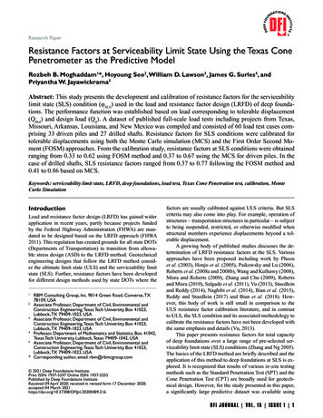
Moghaddam, Seo, Lawson, Surles, Jayawickrama Resistance Factors at Serviceability Limit State Using the Texas Cone Penetrometer as thePredictive ModelgSLS Qδtol – Qd (4)From results of a full-scale load test, the relationship betweenloads applied to the foundation and their corresponding displacements can be expressed by the load-settlement curve.From this curve, Qδtol and Qd can be determined. Conceptually, Qδtol can be regarded as an SLS capacity for a prescribedtolerable displacement. Under conditions presented in Equation (4), a satisfactory performance function is obtained whenQδtol is greater than Qd. Figure 3 is a graphical representationof the concept described and expressed by Equation (4). Alsoshown are the loads and displacements associated with theULS condition as defined by Davisson’s criterion, and 5%and 10% relative settlement criterion.Tolerable Displacement ( δtol )The magnitude or extent of tolerable displacement may bespecified by regulatory agencies such as AASHTO (2014),it can be determined based on behaviors of similar buildingsand structures (Roberts et al., 2010), or it can be determinedbased on predictive models. The National Cooperative Highway Research Program (NCHRP) Report No. 343 (Barkeret al., 1991) presents guidelines and specifications describingallowable total and differential settlement for transportationstructures.An excessive amount of settlement will cause a structure to reach the SLS conditions and if these settlements arefurther increased, a collapse or failure corresponding to theULS conditions may occur. In order to confirm whether anexcessive settlement is present or not, an indicative parameter is required (Salgado 2008). One of the commonly usedFigure 3. Loads corresponding to tolerable displacement (Qδtol) anddisplacement from design loads (Qd) Deep Foundations Institute indicative parameters is the angular distortion (α) which isdefined as the ratio of the differential settlement (δ) to thespan length (L):α δ (5)LIn a study completed by Skempton and McDonald (1956), atotal of 98 buildings consisting of frame buildings and masonry buildings with load bearing walls located in London,England, were selected and analyzed. For each building, relevant information regarding displacement was gathered anda database was compiled based on the type of building. Inaddition to the available information, laboratory testing onreinforced concrete frames and brick walls were carried outunder different angular distortion until cracking happened.Synthesis of the results from the combination of the observeddata and laboratory testing suggested an angular distortionof 0.0033 to reach SLS conditions, 0.006 to experience ULSconditions, and 0.002 for the prevention of both SLS andULS conditions (Salgado, 2008).Burland and Wroth (1974) followed the initial workcompleted by Skempton and McDonald (1956) where theexcessive settlement was assessed based on visible crackson structural elements and determined that a cracking pattern is not always an appropriate method to assess and define an excessive settlement. According to Salgado (2008),visible cracking on structural elements could be an indicator of presence of settlements but not an indication of ULSor SLS condition. Instead of the assessment of crackingpatterns, Burland and Wroth (1974) introduced the beamanalogy where a beam with known span length, height, andelastic properties underwent different loading patterns untilcracking started at different locations on the beam. Basedon the beam analogy, the ratio of the displacement at thecenter of the structure to the length of the structure was recommended as the angular distortion. Results obtained fromthe study completed by Burland and Wroth (1974) werecompared to the angular distortion proposed by Skemptonand McDonald (1956) and it was concluded that the angulardistortion of 0.002 was suitable to prevent both ULS andSLS condition.Zhang and Ng (2005) obtained detailed information regarding displacement of structures located in Hong Kongand China and combined the results with the data publishedby Skempton and McDonald (1956) and Grant et al. (1974)for buildings, and Moulton (1985) for bridge foundations.The final dataset associated with the bridge foundations reported by Zhang and Ng (2005) consisted of 50 concretebridge foundations with angular distortions ranging from0.001 to 0.08. According to Zhang and Ng (2005), 41 bridges were considered tolerable cases where the prescribedfunction of the structure was not affected by angular distortion, and the remaining nine bridges were reported asintolerable cases where the serviceability of the bridge wassignificantly affected. Furthermore, 25 out of 41 bridgesrepresenting 61% of the tolerable cases presented angulardistortions smaller than or equal to 0.002. For intolerableDFI JOURNAL VOL. 15 ISSUE 1 5
Moghaddam, Seo, Lawson, Surles, Jayawickrama Resistance Factors at Serviceability Limit State Using the Texas Cone Penetrometer as thePredictive Modelcases, 78% of these had angular distortions greater than orequal to 0.01.Based on the definition of angular distortion and thework presented by Zhang and Ng (2005) and others, relativeto span length (L), the tolerable displacement of a structurecan be predicted using Equation (6).δtol (6)L 0.002This present study will use the angular distortion of 0.002 toobtain tolerable displacement for subsequent analyses.Development of SLS Resistance FactorsEquations (3) and (4) represent two alternative forms of performance functions for the SLS condition. These equationsmay be identified as the displacement approach and the loadapproach, respectively. Both equations have been used fordevelopment of resistance factors in literature. According toVu (2013), Equations (3) and (4) have equal credibility andthe choice of which approach to use is directly associatedwith data availability.Displacement ApproachIn the geotechnical design process, the resistance is determined based on geotechnical information obtained from fieldand laboratory tests with some level of uncertainties. A design governed by SLS conditions will also be influenced byuncertainties associated with the prediction of displacements.Therefore, uncertainties can be expressed by a resistance factor φ for the SLS condition (φSLS) to further reduce the tolerable displacement and compare the reduced tolerable displacement ( φSLSδtol) to the displacement δd under design load. Forsatisfactory SLS design, the factored tolerable displacement(i.e., reduced tolerable displacement) must be greater than thedisplacement under design load as shown below:φSLSδtol δd (7)Alternatively, Paikowsky and Lu (2006) and Honjo et al.(2005) approached the LRFD methodology at SLS by factoring the displacement presented under design loads (δd). Inthis case, the factored displacement ( φdδd), i.e. the increaseddisplacement under design load, must be smaller than the tolerable displacement as follows:δtol φd δd (8)From Equations (7) and (8), it is noted that in both cases,factors are applied to displacements. In the case of Equation(7), the tolerable displacement is factored and intuitively theresistance factor φSLS is less than unity. On the other hand, thefactor φd is greater than unity to increase the displacementsunder applied design loads, Equation (8).Wang and Kulhawy (2008) explored the developmentof resistance factors at SLS condition using Monte Carlosimulation (MCS). The statistics of tolerable displacements6 DFI JOURNAL VOL. 15 ISSUE 1 reported by Zhang and Ng (2005) were used by Wang andKulhawy (2008) to establish a displacement-based comparison similar to Equation (7) and calibrate resistance factors.Vu (2013) developed resistance factors at SLS condition for the design of drilled shafts installed in shales usinga factored strength parameter approach for the calibrationprocess and the use of displacement based method, Equation(7), where tolerable displacement and design displacementwere variables of the performance function. An appropriateload transfer model for drilled shafts in shales was identified(Vu, 2013) using the “t-z” and “q-z” analysis and variabilitiesand uncertainties associated with the model were quantified.MCS was implemented (Vu, 2013) to develop resistance factors.Load ApproachAs previously mentioned, the SLS performance function canbe expressed in terms of loads, as per Equation (4). In thiscase, in order to account for uncertainties carried during thedesign process, a resistance factor is applied to the load corresponding to the tolerable displacement (Qδtol). Following theLRFD methodology, the factored Qδtol has to be greater thanor equal to the design load (Qd) to ensure satisfactory performance under SLS conditions as shown in Equation (9).φSLS Qδtol Qd (9)The load-based approach for the calibration of resistance factors for the SLS condition has been used by several researchers. Each study has contemplated a unique case and dataset toachieve resistance factors at SLS condition.Phoon et al. (2003) explored the design of drilled shaftsin medium, stiff and very stiff clays, and developed resistancefactors for the SLS condition. A performance function wasproposed and analyzed following the form shown in Equation (9) where the load corresponding to tolerable displacement was factorized and compared to the nominal designload. Similarly, Roberts et al. (2008a and 2008b) and Misraand Roberts (2009) performed a series of research studies focusing on the behavior of drilled shafts at SLS and developedresistance factors for the SLS conditions using MCS methodand following the form of Equation (9).The load-based approach was selected for this presentstudy, and the calibration process for the development ofresistance factors at SLS condition follows the expressionshown in Equation (9).Calibration of Resistance FactorsIn the LRFD methodology, several methods can be used tocalibrate resistance factors. Two of the widely used methodsare the First Order Second Moment (FOSM) and the MonteCarlo Simulation (MCS), see Baecher and Christian (2003)and Fenton and Griffiths (2007). According to Allen et al.(2005), prior to the determination of resistance factors (φ),it is important to understand the statistical distribution of thebias (λ) defined as the ratio of measured resistance (RM) andpredicted resistance (RP), Equation (10). Deep Foundations Institute
Moghaddam, Seo, Lawson, Surles, Jayawickrama Resistance Factors at Serviceability Limit State Using the Texas Cone Penetrometer as thePredictive ModelλR RM (10)RPIn the case of deep foundations and calibration process ofthe resistance factor, the measured resistance (RM) can be determined from results of a full-scale load test; whereas, thepredicted resistance (RP) is obtained from results of predictive models. The statistical distribution of the bias will aid toselect the appropriate method for the calculation of resistancefactors.For calibration process of SLS resistance factors (φSLS),the measured resistance RM is replaced by the load corresponding to tolerable displacement Qδtol which is determinedfrom the load-settlement curves, and the predicted resistanceRP is replaced by design load Qd predicted using any predictive model. For the study presented in this paper and basedon data availability, the TCP design method was selected toobtain design load (Qd).Research Design and MethodDataset DevelopmentThe calibration process of resistance factors is directly a function of measured and predicted capacities. Therefore, predictive models used for the design of deep foundations shouldbe paired with the corresponding resistance factors calibratedusing the same predictive model. For example, if resistancefactors are calibrated based on predicted capacities obtainedfrom a SPT-based method, then those resistance factors areonly applied to SPT-based design method. In a recent TxDOT-sponsored research project assessing the reliability ofthe TCP foundation design method, Seo et al. (2015a, 2015b,2015c) presented the development of resistance factors at theULS conditions. The dataset from that study was used for theSLS analyses presented in this paper.Load Tests and TCP BoringsThe Seo et al. (2015a, 2015b, 2015c) dataset consisted of60 load test cases with corresponding TCP borings. Thesefull-scale load test data were obtained fr
Texas Cone Penetration Test Description of TCP test The TCP test is a dynamic field penetration test which as-sesses the penetration resistance of the material encountered during geotechnical exploration. This test method is docu-mented as TxDOT Designation Tex-132-E, "Test Procedure for Texas Cone Penetration" (TxDOT, 1999) and is formal-