Transcription
Building blocksDiagnosticsSummaryGLM Residuals and DiagnosticsPatrick BrehenyMarch 26Patrick BrehenyBST 760: Advanced Regression1/24
Building blocksDiagnosticsSummaryResidualsThe hat matrixIntroductionAfter a model has been fit, it is wise to check the model tosee how well it fits the dataIn linear regression, these diagnostics were build aroundresiduals and the residual sum of squaresIn logistic regression (and all generalized linear models), thereare a few different kinds of residuals (and thus, differentequivalents to the residual sum of squares)Patrick BrehenyBST 760: Advanced Regression2/24
Building blocksDiagnosticsSummaryResidualsThe hat matrix“The” χ2 testBefore moving on, it is worth noting that both SAS and Rreport by default a χ2 test associated with the entire modelThis is a likelihood ratio test of the model compared to theintercept-only (null) model, similar to the “overall F test” inlinear regressionThis test is sometimes used to justify the modelHowever, this is a mistakePatrick BrehenyBST 760: Advanced Regression3/24
Building blocksDiagnosticsSummaryResidualsThe hat matrix“The” χ2 test (cont’d)Just like all model-based inference, the likelihood ratio test isjustified under the assumption that the model holdsThus, the F test takes the model as given and cannotpossibly be a test of the validity of the modelThe only thing one can conclude from a significant overall χ2test is that, if the model is true, some of its coefficients arenonzero (is this helpful?)Addressing the validity and stability of a model is much morecomplicated and nuanced than a simple test, and it is herethat we now turn our attentionPatrick BrehenyBST 760: Advanced Regression4/24
Building blocksDiagnosticsSummaryResidualsThe hat matrixPearson residualsThe first kind is called the Pearson residual, and is based onthe idea of subtracting off the mean and dividing by thestandard deviationFor a logistic regression model,yi π̂iri pπ̂i (1 π̂i )Note that if we replace π̂i with πi , then ri has mean 0 andvariance 1Patrick BrehenyBST 760: Advanced Regression5/24
Building blocksDiagnosticsSummaryResidualsThe hat matrixDeviance residualsThe other approach is based on the contribution of each pointto the likelihoodFor logistic regression,X {yi log π̂i (1 yi ) log(1 π̂i )}iBy analogy with linear regression, the terms should correspondto 21 ri2 ; this suggests the following residual, called thedeviance residual:pdi si 2 {yi log π̂i (1 yi ) log(1 π̂i )},where si 1 if yi 1 and si 1 if yi 0Patrick BrehenyBST 760: Advanced Regression6/24
Building blocksDiagnosticsSummaryResidualsThe hat matrixDeviance and Pearson’s statisticEach of these types of residuals can be squared and addedtogether to create an RSS-like statisticCombining the deviance residuals produces the deviance:XD d2iwhich is, in other words, 2 Combining the Pearson residuals produces the Pearsonstatistic:XX2 ri2Patrick BrehenyBST 760: Advanced Regression7/24
Building blocksDiagnosticsSummaryResidualsThe hat matrixGoodness of fit testsIn principle, both statistics could be compared to the χ2n pdistribution as a rough goodness of fit testHowever, this test does not actually work very wellSeveral modifications have been proposed, including an earlytest proposed by Hosmer and Lemeshow that remains popularand is available in SASOther, better tests have been proposed as well (an extensivecomparison was made by Hosmer et al. (1997))Patrick BrehenyBST 760: Advanced Regression8/24
Building blocksDiagnosticsSummaryResidualsThe hat matrixThe hat matrix for GLMsAs you may recall, in linear regression it was important todivide by 1 Hii to account for the leverage that a pointhad over its own fitSimilar steps can be taken for logistic regression; here, theprojection matrix isH W1/2 X(XT WX) 1 XT W1/2 ,1/2where W1/2 is the diagonal matrix with Wii Patrick BrehenyBST 760: Advanced Regression wi9/24
Building blocksDiagnosticsSummaryResidualsThe hat matrixProperties of the hat matrixIn logistic regression, π̂ 6 Hy – no matrix can satisfy thisrequirement, as logistic regression does not produce linearestimatesHowever, it has many of the other properties that weassociate with the linear regression projection matrix:Hr 0H is symmetricH is idempotentHW1/2 X W1/2 X and XT W1/2 H XT W1/2where r is the vector of Pearson residualsPatrick BrehenyBST 760: Advanced Regression10/24
Building blocksDiagnosticsSummaryResidualsThe hat matrixStandardized residualsThe diagonal elements of H are again referred to as theleverages, and used to standardize the residuals:ri1 Hiididsi 1 Hiirsi Generally speaking, the standardized deviance residuals tendto be preferable because they are more symmetric than thestandardized Pearson residuals, but both are commonly usedPatrick BrehenyBST 760: Advanced Regression11/24
Building out diagnosticsYou may recall that in linear regression there were a numberof diagnostic measures based on the idea of leavingobservation i out, refitting the model, and seeing how variousthings changed (residuals, coefficient estimates, fitted values)You may also recall that for linear regression, it was notactually necessary to refit the model n times; explicitshortcuts based on H were availableThe same idea can be extended to generalized linear models,although we cannot take advantage of the explicit-solutionshortcuts without making approximationsPatrick BrehenyBST 760: Advanced Regression12/24
Building blocksDiagnosticsSummaryDefinitionsPlotsOne-step approximationsThe resulting approximate statistics are said to be one-stepapproximations to the true valuesThe issue is that we can quickly calculate the one-stepapproximations based on the current weights {wi } withoutrefitting anything, but to calculate the exact value, we wouldneed to go through n IRLS algorithmsThe approximations are usually pretty good, although if onepoint has a very large influence, then the approximation maybe quite different from the true valuePatrick BrehenyBST 760: Advanced Regression13/24
Building blocksDiagnosticsSummaryDefinitionsPlotsOne-step approximationsOne-step approximations allow us to quickly calculate the followingdiagnostic statistics for GLMs:Studentized deleted residuals β (for assessing the change in individual coefficients)Cook’s distance (for assessing overall influence over the modelfit)Patrick BrehenyBST 760: Advanced Regression14/24
Building blocksDiagnosticsSummaryDefinitionsPlotsVariance inflation factorsIt is worth mentioning variance inflation factors (VIF) brieflyhereVIF is a function of X alone, and therefore how VIF iscalculated and what it means is essentially equivalent to thelinear regression case (“essentially equivalent” because we dohave weights for GLMs)In R, we can use the vif function from the car package: vif(fit)AgeSexAge:Sex7.416253 14.159377 16.989516In SAS, this is a bit painful, as we have to use PROC REG,which doesn’t support the CLASS statement or interactions inthe MODEL statement, and you have to calculate andincorporate the weights manually (see code for the messydetails)Patrick BrehenyBST 760: Advanced Regression15/24
Building nearityIf you believe multicollinearity to be a problem, it is often agood idea to look at the correlation matrix for .040.52Sex0.041.000.82Age:Sex0.520.821.00In this model, we are certainly introducing a lot of variabilityby including an interaction; on the other hand, the interactiondid seem to be important p 0.05Patrick BrehenyBST 760: Advanced Regression16/24
Building blocksDiagnosticsSummaryDefinitionsPlotsLeverageTo get a sense of the information these statistics convey, let’s lookat various plots of the Donner party data, starting with .050.002030405060AgePatrick BrehenyBST 760: Advanced Regression17/24
Building blocksDiagnosticsSummaryDefinitionsPlotsCook’s DistanceDiedSurvived20Female30405060Male0.4Cook's distance0.30.20.10.02030405060AgePatrick BrehenyBST 760: Advanced Regression18/24
Building blocksDiagnosticsSummaryDefinitionsPlotsDelta-beta (for effect of age)DiedSurvived20Female30405060Male β0.040.020.00 0.022030405060AgePatrick BrehenyBST 760: Advanced Regression19/24
Building blocksDiagnosticsSummaryDefinitionsPlotsResiduals / proportional leverage Died Survived 1 6 1 45 30 2 d2(Studentized deleted) 1 2 0.20.40.60.80d(Studentized deleted) 1.0π 0.2 0.40.60.8 1.0πPatrick BrehenyBST 760: Advanced Regression20/24
Building blocksDiagnosticsSummarySummaryResiduals are certainly less informative for logistic regressionthan they are for linear regression: not only do yes/nooutcomes inherently contain less information than continuousones, but the fact that the adjusted response depends on thefit hampers our ability to use residuals as external checks onthe modelThis is mitigated to some extent, however, by the fact that weare also making fewer distributional assumptions in logisticregression, so there is no need to inspect residuals for, say,skewness or heteroskedasticityPatrick BrehenyBST 760: Advanced Regression21/24
Building blocksDiagnosticsSummarySummary (cont’d)Nevertheless, issues of outliers and influential observations arejust as relevant for logistic regression as they are for linearregressionIn my opinion, it is almost never a waste of time to inspect aplot of Cook’s distanceIf influential observations are present, it may or may not beappropriate to change the model, but you should at leastunderstand why some observations are so influentialPatrick BrehenyBST 760: Advanced Regression22/24
Building blocksDiagnosticsSummaryExtubation exampleLeft: Linear cost; Right: Log(Cost)Cook's distance5Cook's distance50100200300Obs. numberPatrick Breheny0.10Cook's distance04194290.00320Cook's distance14191800.203174317050100200300Obs. numberBST 760: Advanced Regression23/24
Building blocksDiagnosticsSummaryVariance inflationFinally, keep in mind that although multicollinearity andvariance inflation are important concepts, it is not alwaysnecessary to calculate a VIF to assess themIt is usually a good idea when modeling to start with simplemodels and gradually add in complexityIf you add a variable or interaction and the standard errorsincrease dramatically, this is a direct observation of thephenomenon that VIFs are attempting to estimatePatrick BrehenyBST 760: Advanced Regression24/24
Deviance and Pearson's statistic Each of these types of residuals can be squared and added together to create an RSS-like statistic Combining the deviance residuals produces the deviance: D X d2 i which is, in other words, 2' Combining the Pearson residuals produces the Pearson statistic: X2 X r2 i Patrick Breheny BST 760: Advanced .