WIXLIB

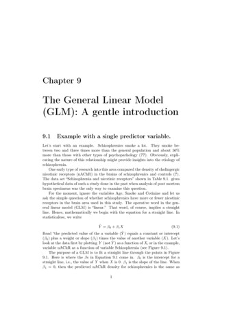
CHAPTER 9. THE GENERAL LINEAR MODEL (GLM): A GENTLE9.3. GLM TERMINOLOGYINTRODUCTIONSchizophrenics smoke more than controls. Because of the amount of missingdata for smoking status at death, the initial brain samples could not be adequately matched for this important variable. Consistent with previous evidence,nicotine up regulated acetylcholine nicotinic receptors and, of course, results inhigh levels of its metabolite cotinine. This up regulation masked the difference in nAChR density between schizophrenic and control brains in the initialanalysis.Hence, the conclusion of this exercise is that schizophrenia is associatedwith decreases in nAChR number. Note carefully that the operative word is“associated ”. Synonyms would be “correlated ” and “predicted.” Finally, notethat any real life analysis would start with the third GLM that used age, cotinineand diagnosis as predictors. The order of presentation for the GLMs above waspurely didactic.9.3GLM terminologyAs in the vocabulary for any system that has evolved over time, GLM terminology can be confusing. As statistical theory grew, it was realized that severaldifferent techniques could be combined into a single, general technique. Hence,the term general in GLM. Also, the advent of digital computers permitted themathematics behind the general approach to be implemented. Nevertheless, weare left with a legacy of terms derived from the old techniques as well as tablesand short cuts used in hand calculations.The first type of terminology applies to the variables in the GLM. Thevariable on the left hand side of the GLM equation (Y or nAChR in the example)is called the dependent, predicted, or response variable. The variables on theright side of the equation (the X s or Schizophrenia, Age, and Cotinine) are calledthe independent, predictor, or explanatory variables. Usually, these terms arepaired: dependent with independent, predicted with predictors, and responsewith explanatory.An independent, predictor or explanatory variable that is measured withnumbers is called a numeric or quantitative variable or a covariate. One that isnot numeric (or uses numbers to indicate groups) is called a factor.2 The specificgroups within a factor are termed the levels of that factor. For example, thefactor sex would have two levels–female and male.The three classic statistical procedures that comprise the GLM are: (1) theanalysis of variance or ANOVA; (2) the analysis of covariance or ANCOVA;and (3) regression. In ANOVA, all of the independent variables are factors(i.e., qualitative variables). An ANOVA with only one factor is called a onewayANOVA. An ANOVA with more than one factor is called a factorial ANOVA.Often a factorial ANOVA is described by the number of levels in the factors.For example, if the first factor has two levels and the second factor has threelevels, the model is called a “two by three” design or “two by three ANOVA.”2 Sometimesnonnumeric variables are called qualitative variables.8

CHAPTER 9. THE GENERAL LINEAR MODEL (GLM): A GENTLEINTRODUCTION9.4. THE MEANING OF THE BETASA regression is GLM in which all of the variables are quantitative. Whenthere is only one X or independent variable, the regression is called a simpleregression. When there are two or more X s, the regression is called a multipleregression.An ANCOVA is a GLM with at least one qualitative and at least one quantitative predictor. Hence, ANCOVA is synonymous with GLM. Most statisticianstoday eschew the term ANCOVA and use GLM.9.3.1Orthogonal and non orthogonal designsIn generic statisticalese, the word orthogonal is a synonym for uncorrelated.Like most jargon in science, it was probably developed for two reasons: (1) lendan air of respectability to statistics as a science; and (2) deliberately confuseanyone trying to learn the field. When all independent variables of a GLM areuncorrelated with one another, then the model is orthogonal. When at least onepair of independent variables are correlated, the design is non-orthogonal. If theGLM has at least one continuous independent variable, then always regard itas non-orthogonal3 . Hence, the term orthogonal only applies to classic ANOVA, i.e., when all independent variables are strictly categorical. An ANOVA isorthogonal when each cell contains the same number of observations. Thiscondition is also termed a balanced design.In an orthogonal design, there is one and only one mathematical way toestimate the parameters of the model and to perform the statistical tests. Innon-orthogonal designs, however, there is more than one way to compute thesestatistics, so the user must make some assumptions about the best way to interpret the results.Finally, orthogonality is not akin to falling off a cliff. A two by two ANOVAthat has eight rats in three of its cells but seven in the fourth is so close tobeing orthogonal that the different ways of estimating the sums of squares willall yield the same substantive results. Hence, most designs in experimentalneuroscience will be close to being orthogonal. The issue is much more salientfor certain types of observational research. A random sample of, say, alcoholicsor sociopaths will contain roughly three males for every female. Here, one mustbe very careful about which type of sums of squares to request and to interpretwhen a variable like gender is in the model. In general, the more correlatedthe independent variables are, the more care must be taken in interpreting theresults.9.4The meaning of the betasThe general equation for GLM isŶ β0 β1 X1 β2 X2 . . . βk Xk3 Thereare exceptions to this rule but they are beyond the scope of this book.9(9.3)

CHAPTER 9. THE GENERAL LINEAR MODEL (GLM): A GENTLE9.4. THE MEANING OF THE BETASINTRODUCTIONThe βs in a GLM are coefficients or weights assigned to the predictor variables, i.e. the X s on the right had side of the prediction equation. Here, let usexplore some properties of these coefficients.The first β, β0 , is a constant. That it, it is the same for every observationregardless of any values on any of the X s. In geometrical terms, β0 is anintercept. Examine Equation 9.3 and let all of the X s equal 0. β0 is thepredicted value of Y when all of the X s equal 0. In terms of our example, itwould be the predicted nAChr density for neonatal controls (age is 0) with nobrain cotinine. (This prediction, however, is not sensible because it extends farbeyond the age range of the observed data, See Section X.X).The other βs are all associated with a variable. Because the variable is multiplied by the β, the β is a “weight” that determines how much the X contributesto prediction. If β 0, then the associated variable does not predict individualdifferences in Y (once again, with the proviso that we are controlling for allthe other variables). As an example, suppose that the β for age had been 0 inthe nicotinic receptor data. Then if we picked a subject with a given diagnosisand cotinine value, then changing age would make no difference in the predictednAChR level for that individual.In more specific terms, a β gives the predicted change in Y for a one unitchange in the X, keeping everything else constant. There is a very simple proofof this interpretation. Assume GLM equation of the form of Equation 9.3 andconcentrate on the ith X. We can write this equation asŶ0 . . . βi Xi(9.4)where the ellipses (. . .) denote “everything else in the equation that is keptconstant.” Now change the value of Xi from Xi to (Xi 1). The predictedvalue is nowŶ1 . . . βi (Xi 1)(9.5)Subtracting Equation for Ŷ0 from that for Ŷ1 from X givesŶ1 Ŷ0 βi (Xi 1) βi Xi βiA β gives the predicted change in Y for a one unit increase in X.Hence, the β for age (-.12) informs us that a one year increase in age isassociated with a decrease of -.12 units of brain nAChR. The β for cotinine tellsus that a one unit increase in cotinine predicts .08 units of increase in nAChR.Finally, an increase in one unit of diagnosis (in effect, a change from control toschizophrenia) predicts -5.7 units decrease in nAChR.Note carefully that the actual magnitude of a βs is a function of the unitsof measurement of its X. Suppose X was measured in milligrams. The β wouldgive the predicted change in Ŷ for a one milligram increase in X. If we changed10

CHAPTER 9. THE GENERAL LINEAR MODEL (GLM): A GENTLEINTRODUCTION9.4. THE MEANING OF THE BETASthe scale of X from milligrams to micrograms, then the β in the new equationwould give the change in Ŷ from a one microgram change in X. One can thereforearbitrarily make a β larger or smaller by simply changing the scale of its variable.This scale property of β leads to one of the most important cautions ininterpreting the results from a GLM: never compare the βs across variables todetermine the importance of the variables in prediction. In our example, theβ for a diagnosis of schizophrenia was -5.7 while the one for cotinine was .08.This does NOT imply that schizophrenia predicts nAChR much better thancotinine. Statistics other than the βs must be used to compare the effect sizesof the predictors.Never compare βs across variables to determine the importance of thevariables in prediction.9.4.1Standardized betasThe type of betas (βs) that we have been dealing with are often called raw orunstandardized regression or GLM coefficients. These terms derive from thefact that the predictor variable are expressed in raw or unstandardized units.In some cases, it is helpful to examine standardized regression coefficients.Suppose that we transformed the response variable, Y, to a new variable,ZY , with standard scores (see Section X.X). This means that the mean of ZY is0 and the variance of ZY is 1.0. Suppose that we also standardized each of thepredictor variables in the model to have means of 0 and standard deviations of1. The GLM equation isZŶ β0 β1 ZX1 β2 ZX2 . . . βk ZXk(9.6)The βs in this equation are called standardized coefficients. They are the GLMcoefficients from a model in which all variables have been standardized to havea mean of 0 and a standard deviation of 1.0.Standardized βs may be used to compare the relative predictive effectsof the independent variables.The interpretation of a standardized coefficient is the same as the one fora raw β but is expressed in terms of standard deviation units instead of rawunits. Hence, if β1 .09, then we predict that a one standard deviation changein variable X1 will result in a .09 standard deviation change in Y. Because all ofthe standardized predictor variables are the in the same units, standardized βsmay be compared to assess the predictive effect of one variable versus another.11

CHAPTER 9. THE GENERAL LINEAR MODEL (GLM): A GENTLE9.5. GLM AND CAUSALITYINTRODUCTIONThat is, if the standardized β1 .12 and standardized β2 .07, then X1 is abetter predictor of Y than X2 .9.5GLM and causalityIt is essential to stress that even though we speak of “dependency”, “explanations” and “effects,” causal interpretation of a GLM depends on the design ofthe study. True experiments (i.e., direct experimental manipulation, randomassignment, and strict control) permit inferences about causality. Given appropriate controls, if manipulation of variable A results in a change in the dependentvariable, then in some way, shape or form–directly or indirectly–A has a causalinfluence on the response. How that causal influence comes about, whether therelationship is necessary and/or sufficient, and the mechanism(s) of causalitycannot be answered by the statistical analysis of an experiment. Often, the answer to these questions depends on substantive issues coupled with the outcomeof the experiment.The smoking example is an excellent one for the discussion of causality.Cotinine predicts receptor density, but does it cause change in the numberof receptors? Probably not. The most likely casual agent is nicotine. Thenicotine up regulates receptors (?) and generates cotinine as a metabolite.Hence, cotinine is correlated with but has little causal effect on the number ofreceptors. Because of cotinine’s long half life (relative to nicotine), it works asa good control variable in the study.Technically, a GLM applied to non-experimental observational research doesnot permit inferences about causality. But one must be reasonable here becauseinterpretation of a GLM must be taken in the context of existing data andtheory. There has never been, and never will be, a true experiment examiningthe health consequences of cigarette smoking in humans. It would be unethical–in fact, downright cruel–to randomly assign young adolescents to a smokinggroup and a non-smoking control group, compelling the former to smoke and thelatter to abstain from cigarettes, until their health status could be ascertained40 years later. Yet, all the observational, epidemiological data on humans agreeso well with true experiments in animals and with mechanistic research into thecardiovascular and pulmonary effects of smoking that reasonable scientists infera causal connection.12

Chapter 9 The General Linear Model (GLM): A gentle introduction 9.1 Example with a single predictor variable.