Transcription
Polymer Processing Simulations TrendsTim A. Osswald, University of Wisconsin-MadisonPaul J. Gramann, The Madison Group-PPRCMadison, WI, USA1IntroductionIn most polymer processes the quality of the final part is greatly dependent onthe melting, flow and mixing of the polymer. The optimization of the equipmentand manufacturing process, as done today, is time consuming and expensive.Quantifying flow and heat transfer is an even more intimidating task.Furthermore, reproducing the properties of a particular blend from batch to batch,or part performance from shift to shift, can be extremely difficult. Obviously thesebarriers make numerical simulation of polymer processes a viable alternativewhen optimizing and analyzing the process.Traditionally, when simulating polymer processes the main concern of theengineer has been to accurately represent the material behavior using complexmodels. Although many problems still exist regarding polymer material models,today one can easily deal with the shear thinning behavior, temperaturedependence and to some degree the viscoelasticity of polymers. In fact, to date alarge number of processes have been realistically simulated in polymerprocessing ranging from mold filling with fiber orientation, shrinkage and warpageto extrusion with viscoelastic effects. However, only a few fully three-dimensionalmodels of realistic processes have been solved. Simulating a fully threedimensional process involves intensive labor trying to accurately represent thegeometry of the device and also requires large amounts of computation and datastorage. Obviously, computational demands have been dampened by theenormous increase in computational power available to the engineer at thedesktop. The labor intensity and requirements of computer performance aremultiplied by the added complexity of moving boundaries. There are two types ofmoving boundaries that are very common in polymer processing: moving freeboundaries and moving solid boundaries. Moving free boundary problems areencountered in mold filling, extrudate swell, coating problems, inside the extruderat the screw, to name a few. Solid moving boundaries are those where the actualcavity that contains the polymer changes in shape during the process, i.e. therotating mixing heads in an internal batch mixer or the screw and mixingelements in a single screw extruder. An assumption that the device is completelyfilled with melt is taken, which may not always be realistic The most complexprocess that involves solid moving boundaries is the intermeshing twin screwextruder. Here, the domain of interest, i.e. the polymer, is constantly changingshape as the screws, mixing heads and kneading blocks rotate. The self-wipingarrangement of these systems adds to the complexity of the problem, since itinvolves very small gaps, which introduce numerical complications. One shouldregard the complete simulation of the twin screw extrusion processes including
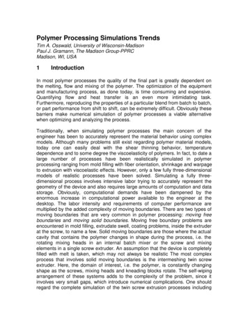
Polymer Processing Simulation Trends2melting, melt conveying, mixing, die flow to the prediction of final morphology,including coalescence and a partially filled system, should be regarded as one ofthe grand challenge problems in polymer processing.The advent of more powerful computers and efficient numerical techniques arenow beginning to make it possible to simulate three-dimensional problems ofcomplex geometry with non-linear material behavior.This paper presents a general overview of the state-of-the art techniques usedfor the modeling and simulation of polymer processes. A brief background onnumerical techniques and basic modeling in polymer processing is presented. Adiscussion on two-dimensional models that are used to simulate threedimensional flows is followed by recent advancements in full three-dimensionalmodels.2. RheologyMost polymer processes are dominated by the shear strain rate. Consequently,the viscosity used to characterize the fluid is based on shear deformationmeasurement devices. The rheological models that are used for these type offlows are usually termed Generalized Newtonian Fluids (GNF). In a GNF modelthe stress in a fluid is dependent on the second invariant of the stain rate tensor,which is approximated by the shear rate in most shear dominated flows. Thetemperature dependence of GNF fluids is generally included in the coefficients ofthe viscosity mode. The shear viscosity of a typical polymer melt is shown in Fig.1. Various models are currently being used to represent the temperature andstrain rate dependence of the viscosity.Figure 1. Shear viscosity curve for LDPE
Polymer Processing Simulation Trends3The power law model is a simple model that accurately represents the shearthinning region in the viscosity curve, but neglects the Newtonian plateau at smalland large strain rates. The major disadvantage of this model is that the viscositygoes to infinity at low stain rates and zero at high strain rates. The infiniteviscosity leads to erroneous results in problems where there is a region of zeroshear rate, such as in the center of a tube. However, this problem can beovercome by using a truncated model where a constant viscosity is assumed inthe strain rate region of Newtonian behavior.A model that fits the complete range of strain rate is one developed by Bird andCarreau [1]. The Bird-Carreau model accurately models the Newtonian plateauobserved at low and sometimes high strain rates, and the shear thinning regionin-between.The Bingham model represents the rheological behavior of materials that exhibita “no flow” region below certain yield stresses, such as polymer emulsions,slurries and some food products such as ketchup. Above a yield stress thematerial flows like a Newtonian liquid.The tendency of polymer molecules to “curl-up” while they are being stretched inshear flows results in normal stresses in the fluid that greatly affect the flow fieldin certain cases. Additionally, most polymer melts exhibit an elastic as well as aviscous response to strain. This puts them under the category of viscoelasticmaterials. There are no precise models that accurately represent this behavior inpolymers. However, various combinations of elastic and viscous elements havebeen used to approximate the material behavior of polymer melts1. Some modelsare combinations of spring and dashpots to represent the elastic and viscousresponses, respectively. The most common ones being the Maxwell model for apolymer melt and Kelvin or Voight model for a solid. One model that representsshear thinning behavior, normal stresses in shear flow and elastic behavior ofcertain polymer melts is the K-BKZ model [2-3].Elongational of “shear-free” flows are the least studied types of flows that occurin polymer processing. A major reason for this is that they are not as common asshear flows that dominate extrusion and injection molding. However, in certainpolymer processes, such as fiber spinning, blow molding, thermoforming,foaming and compression molding, under specific processing conditions, themajor mode of deformation is elongational. Moreover, the elongational viscositythat is needed for simulation is difficult to measure and thus requires expensiveequipment.1For a more detailed presentation concerning rheological models the reader is referred to Bird, R.B., R.C.Armstrong and O. Hassager, Dynamics of Polymeric Liquids, Vol. 1, Wiley, New York (1987). In addition,Bird and Wiest give a complete review paper on models available to model viscoelastic behavior ofpolymer melts in Bird, R.B., and J.M. Wiest, "Constitutive Equations for Polymeric Liquids," Annu. Rev.Fluid Mech., 27, 169-93, 1995.
Polymer Processing Simulation Trends43. ModelingIn order to be able to predict and model complex polymer flows, one must firsthave a basic understanding of the mathematics that govern the flow. Regardlessof the complexity of the flow, it must satisfy certain physical laws. These laws canbe expressed in mathematical terms as the conservation of mass, theconservation of momentum, and the conservation of energy. In addition to thesethree conservation equations, there may also be one or more constitutiveequations that describe material properties, i.e. shear thinning behavior. Sincethese equations may also be coupled together, i.e. temperature dependentviscosity, the solution can become even more complex. The goal of the modeleris to take a physical problem, apply these mathematical equations and solvethem to predict the flow phenomena. Although analytical solutions to theconservation equations for some simple two-dimensional shapes are available,when more complex two-dimensional problems or three-dimensional analysis arerequired, numerical methods are required. There are three basic classes ofnumerical techniques that are commonly used to solve complex fluid flowproblems (Fig.2). They are: the finite difference method (FDM), the finite elementmethod (FEM), and the boundary element method (BEM). Each of thesemethods has its own advantage and disadvantages and, therefore, one may bepreferred for certain type of process or material. Each technique has beenadapted in some form for specific problems encountered in polymer processing.Figure 2. Comparison between various numerical techniques
Polymer Processing Simulation Trends53.1 Finite Difference MethodThe finite difference method started gaining prevalence in the 1930’s for use inhand calculations and is the simplest to use and understand. Figure 2 shows thegrid that would be constructed to represent the geometry of a two-dimensionaldomain. Once the grid is created, the governing differential equations arerewritten in a discretized form and then applied at each nodal point. The resultingsystem of algebraic equations can then be solved for by standard Gaussianelimination or more elaborate numerical algorithms. Because of the simplicity ofthe method, it can implemented in a wide variety of problems. The methoddiscretizes the governing equations at the start of the analysis, and it lends itselfto model non-linear problems. The finite difference method is also easy toprogram and computer simulations can provide quick computation times. Thefirst consideration when implementing the FDM is that it is best suited for casesthat have relatively simple geometries. Even though more complex geometriescan be modeled with special differential equations or coordinate transformations,there are still limitations that exist, and the other methods presented in this paperoften prove to be more efficient. However, for a quick assessment of a process orproduct performance, often a 1D simplication of the process can yield usefulresults. Such is the case with the simplified solution of injection mold fillingpresented in Fig.3.Figure 3. Flow length, flow rate and pressure prediction during injection moldingusing a 1D FDM simulation program.3.2 Finite Element MethodIn contrast to the FDM the finite element method is a relatively new techniqueused for solving fluid flow problems. Popularized in the 1960’s along with theadvent of digital computers, the finite element method has become the basis formost commercial structural dynamic and fluid flow simulation programs. Like
Polymer Processing Simulation Trends6FDM, FEM is a domain method in which the entire geometry to be modeled mustbe discretized into nodes and elements. The mesh shown in Fig. 2 representsthe discretization required for FEM to model a two-dimensional geometry.Although several different methods are available to obtain the final equations, theGalerkin method of weighted residuals is normally preferred in fluid flowproblems. Once the mesh has been created, the governing differential equationsare then expressed in integral form and numerically integrated to obtain analgebraic system of equations. Because of the nature of the finite elementmethod, it is capable of modeling much more complex geometries than FDM. Itcan also provide quite accurate solutions to the field variables, such as fluidvelocities or pressures, for a wide variety of problems that include non-linearflows. However, higher order derivative solutions, such as velocity gradients,tend to be less accurate. Without complex adaptive meshing techniques, FEM isalso difficult to use for problems with moving solid boundaries. Since thegoverning equations are approximated with the Galerkin method, they have acertain amount of intrinsic error even before numerical errors are accounted for,which is carried throughout the computation. This can cause the FEM to becomeunstable in highly non-linear situations. Although this can be partially alleviatedby special upwinding techniques it nonetheless increases the amount ofcomputation effort. In addition, since the solution is computed only at the nodesand the velocity field must be interpolated, the tracking of particles in the flowfield in not easily accomplished with FEM.However, FEM is extensively used when simulating processes that are highlynon-linear such as flow of viscoelastic materials. For example, Fig.4 showspredicted extrudate swell of HDPE flowing through a converging die [4]. Mitsoulis[4] predicted the flow of various materials through dies of different geometryusing the K-BKZ model. His numerical results compared well with experiments.Figure 4. Predicted extrudate swell of HDPE flowing through a converging die.
Polymer Processing Simulation Trends7The finite element has also proved to be ideal when simulating mold fillingprocesses, fiber orientation, shrinkage and warpage of thin plastic parts. Themajor difficulty which arises when simulating molding processes (and othermoving boundary processes) is tracking the transient free surface (or solidmoving boundaries during mixing). The material constantly changes shape as itflows and is deformed inside the cavity, making it necessary to redefine thegeometry of the domain of interest after each successive time step. Redefiningthe finite element mesh or finite difference grid is the most tedious part ofsimulations when dealing with moving boundary problems and many timesmakes it unreasonable to simulate.Kouba and Vlachopoulos [5] and deLorenzi and Nied [6] developed a techniqueto model membrane stretching during blow molding and thermoforming. Althoughthe processes are basically three-dimensional, they can be represented with twodimensional plate elements oriented in three-dimensional space.Tadmor, Broyer and Gutfinger [7-8] used a spatial finite difference formulation tosolve two-dimensional flow problems in complex geometrical configurations.Using a Hele-Shaw [9] formulation to simulate the flow; their method is applicableto flows in narrow gaps of variable thickness, such as injection molding of thinparts and flows inside certain extrusion dies. This technique is known as the flowanalysis network (FAN), and works well for Newtonian and non-Newtonian fluids.The method uses an Eulerian grid of cells that covers the flow cavity. A fill factoris associated with each cell, a number that varies between zero and one. A fillfactor denotes an empty cell, and a fill factor of one denotes a cell that is full ofmaterial. A local mass balance is made around each cell, which results in a set oflinear algebraic equations with pressures at the center of the cells as theunknown parameters. The pressure field that results from solving the set ofequations is used to calculate the flow distribution between the cells, which inturn is used to advance the flow inside the cavity by updating the cell fill factors.A major disadvantage of this technique is that relatively fine meshes arerequired, especially if curved boundaries are present in the geometry. Thisdisadvantage can be overcome by using finite difference operators, however, thismakes the simulation awkward and difficult to use.Osswald and Tucker [10] and Wang et al. [11] modified the flow analysis networkto model the non-isothermal flow of non-Newtonian fluids inside thin threedimensional cavities using finite elements. The technique, which is commonlyknown as the control volume approach (CVA) requires that the three-dimensionalmolding surface be divided in flat three- or four-noded finite elements. Cells orcontrol volumes are generated by connecting element centroids with elementmid-sides. When applying the mass balance to each cell, the resulting equationsare the same than those that result from applying the Galerkin method to thegoverning equation for pressure. This allows the use of standard finite elementassembling techniques when generating the set of liner algebraic equation. Atypical configuration of elements and nodal control volume is shown in Fig. 5. In
Polymer Processing Simulation Trends8the figure the solid lines denote element sides and the dashed lines represent thecontrol volume boundaries. The hashed area represents the control volume fornode i. This technique remains the dominant form of modeling mold fillingprocesses such as compression and injection molding.Figure 5. Finite element / control volume configurationCommercially available software packages all use this technique to track the flowfronts during mold filling. As an example Fig. 6 presents the mold filling patternduring mold filling of a compression molded SMC part represented with the meshshown in Fig.7. Figure 8 presents the fiber orientation distribution within thecompression molded fender shown in Figs.6-7. Mold filling simulation programshave shown good agreement with experimental results. Work still needs to bedone when predicting mold filling of very thin injection molded products. Sincethe industry is constantly reducing part thickness, this issue remains a topresearch priority for the injection molding community.
Polymer Processing Simulation TrendsFigure 6. Simulated mold filing pattern during compression molding of anautomotive SMC fender.Figure 7. Finite element mesh of the automotive fender9
Polymer Processing Simulation Trends10Figure 8. Fiber orientation prediction within the compression mold automotivefender3.3 Boundary Element MethodIn contrast to both the finite difference and finite element methods, the boundaryelement method (BEM) only requires that the boundary or surfaces of thegeometry be discretized. As shown in Fig. 2, a two-dimensional geometry onlyrequires a discretization of the curve that makes up the boundary of the part. Inessence, the order of analysis being made is reduced by one. Figure 9 comparesFEM and BEM discretizations of a two dimensional model of an internal batchmixer [12].BEM also gained prevalence around the same time as FEM, but because of therelatively complex mathematics involved with BEM, it has been relatively slow togain the same level of acceptance that FEM did in the engineering community,and has been primarily used by mathematicians. The formulation of the boundaryelement method begins with a different form of the governing equations, whichare expressed in terms of domain integrals. These integrals are manipulated byGreen-Gauss transformations until they are reduced to boundary integrals. Theintegrals are then numerically evaluated to yield an algebraic system ofequations. Interestingly, up to the point of evaluating the integrals, noapproximations have been made in the governing equations. Thus, the boundaryelement method, unlike the FDM or FEM, does not introduce any error to thesolution until the boundary is discretized – the boundary element solution is exactup until the geometry is meshed. Another advantage of BEM is that the accuracyof higher order derivatives is excellent. This becomes extremely important whentrying to calculate heat transfer effects or track particles. Here, the boundaryelement is well suited to track particles in the flow of material since the solution atany location in the fluid can be obtained quite easily and very accurately.
Polymer Processing Simulation Trends11130 nodes4921 nodesFigure 9. BEM and FEM discretization of a 2D (completely filled) internal batchmixerA typical simulated mixing history inside the above internal batch mixer ispresented in Fig. 10[13]. It is important to point out that, up to date, all mixinganalyses performed on internal batch mixers assume a full mixing cavity.However, a mixing process greatly depends on the fill factor of the mixer. Thisremains an area of research of the polymer processing research community, andcan be eventually addressed using BEM.
Polymer Processing Simulation Trends12Figure 10. Simulated domain deformation during mixing.Other areas where BEM is being applied are complex three dimensional flowssuch as shown in Fig.11 below. Here, a double flighted co-rotating twin screwextruder was simulated using a 3D BEM simulation {Krawinkel]. Although BEMhas proven very versatile when dealing with complex geometries, the techniqueis still primarily being used to simulate linear problems such as linearly elasticstress strain problems or Newtonian flow problems. However, research isunderway to simulate non-linear problems with BEM and still maintain theboundary only discretization. Since BEM generates full unsymmetric matrices itdoes not bring a great gain in computational savings. However, the greatestadvantage of BEM is the ease with which a complex geometry is generated andsimulated, significantly reducing problem preparation time and practicallyeliminating the need of user interaction.
Polymer Processing Simulation Trends13Figure 11. Pressure distribution on the screw surfaces and particle trajectoriesinside a twin screw extruder.4. References1. Carreau, P.J., Ph.D. Thesis, University of Wisconsin-Madison, 1968.2. Kaye, A., College of Aeronautics, Cranfield, Note 134, 1962.3. Bernstein, B., E. Kearsley and L. Zapas, Trans. Soc. Rheology, 7, 391-410,1963.4. Luo, X.-L., and E. Mitsoulis, J. Rheol., 33, 1307, 1989.5. Kouba, K. and J. Vlachopoulos, ANTEC 114-116, 1992.
Polymer Processing Simulation Trends146. DeLorenzi, H.G. and H.F. Nied in "Progress in Polymer Processing," A.I.Isayev, Ed., Hanser Publishers, 1991.7. Tadmor, Z, E. broyer, C. Gutfinger, Polym. Eng. Sci., 14, 660-665, 1974.8. Broyer, E., C. Gutfinger, and Z. Tadmor, Trans, Soc, Rheol., 9, 423-444,1975.9. Hele-Shaw, H.S., Proceed. Royal Inst., 16, 49-64, 1899.10. Osswald, T.A., and C.L. Tucker III, Int. Polym. Process., 5, 79-87, 1990.11. Wang, V.W., C.A. Hieber and K.K. Wang in "Applications of Computer AidedEngineering in Injection Molding," L.T. Manzione, Ed., Hanser Publishers,1987.12. Osswald, T.A., and E. Baur "BEM in der Kunststoffverarbeitung – EinÜberblick (BEM in Polymer Processisng – A Review)," Kunststoffe, 89, 2,1999.13. Hutchinson, B., A.C. Rios and T.A. Osswald ”Modeling the Distributive Mixingin an Internal Batch Mixer," Int. J. Polym. Proc., 16, 315, 1999
storage. Obviously, computational demands have been dampened by the enormous increase in computational power available to the engineer at the . polymer processes, such as fiber spinning, blow molding, thermoforming, foaming and compression molding, under specific processing conditions, the major mode of deformation is elongational. Moreover .