Transcription
Flint Water Crisis: Data-Driven Risk Assessment ViaResidential Water TestingJacob AbernethyCyrus AndersonChengyu .eduArya FarahiLinh NguyenAdam eduEric SchwartzWenbo ShenGuangsha h.eduJonathan StroudXinyu TanJared h.eduSheng Yangphysheng@umich.eduUniversity of MichiganAnn Arbor, MIABSTRACTRecovery from the Flint Water Crisis has been hindered byuncertainty in both the water testing process and the causesof contamination. In this work, we develop an ensemble ofpredictive models to assess the risk of lead contamination inindividual homes and neighborhoods. To train these models,we utilize a wide range of data sources, including voluntaryresidential water tests, historical records, and city infrastructure data. Additionally, we use our models to identifythe most prominent factors that contribute to a high risk oflead contamination. In this analysis, we find that lead service lines are not the only factor that is predictive of the riskof lead contamination of water. These results could be usedto guide the long-term recovery efforts in Flint, minimize theimmediate damages, and improve resource-allocation decisions for similar water infrastructure crises.KeywordsWater Quality, Flint Water Crisis, Risk Assessment, Machine Learning1.INTRODUCTIONThe Flint Water Crisis began in April 2014 when the city ofFlint, Michigan switched its water supply from Lake Huronto the Flint River as a temporary cost-saving measure. Notlong afterwards, the water in many Flint residences wasfound to be contaminated with dangerously high levels oflead. It was discovered that the highly-corrosive water drawnin from the Flint River was not treated with the proper anticorrosive chemicals prior to the switch, causing lead particles to leech into the water supply from the lead pipes thatcomprise much of the city’s aging infrastructure. In manyplaces, the levels of lead in the water exceeded one hundred times the federal actionable level of 15 parts per billion (ppb), and blood-borne lead levels in children increasednoticeably since the switch [10]. Since lead-contaminatedwater poses significant health risks, particularly for children[1], the mayor of Flint declared the city to be in a state ofemergency in December 2015. Flint has since returned tothe water shipped in from Lake Huron. However, lead contamination has yet to return to safe levels. The city of Flintnow faces a daunting infrastructural problem: find whichhomes are most drastically affected by lead contaminationand repair their plumbing systems. Conventional wisdomsays that homes with lead service lines are at the highestrisk of contamination, and it is estimated that Flint hasover 8000 such service lines 1 . This problem has gatheredsignificant national attention, and the city of Flint is nowunder pressure to repair the infrastructural issues as quicklyand efficiently as possible.Although many believe that repairing the lead service lineswill remove lead contamination, there are a number of difficulties that complicate this proposed solution. First, it is notclear whether repairing all of Flint’s lead service lines willeliminate the problem. Even if the contact between corrosive Flint River water and lead service lines was the originalcause of lead contamination, other regions in the water delivery pipeline now contain contaminated water. This watermay remain in the infrastructure if the surrounding watersystems are unused for prolonged periods, and may continueto contaminate nearby residences when fluctuations in waterpressure eventually push it through the system. Flint is particularly at high risk of this phenomenon because it has 870/Bloomberg Data for Good Exchange Conference.25-Sep-2016, New York City, NY, USA.
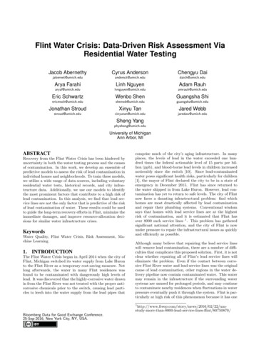
of the highest property vacancy rates in the country. This isjust one of many factors besides lead service lines that mayput a particular home at risk. Understanding the complexrelationship between the contamination problem and features of the infrastructure will allow policymakers to moreeffectively target the problem and minimize damage.able from the state of Michigan, and other components wereprovided by the city at our request, as noted.2.1Residential Lead TestsThe second complication is that it is not clear which homesare most effected by contamination. To address this, thecity has implemented a voluntary residential water testingprogram that allows residents to collect their own water andsubmit it for testing at a local center. However, not allhomes have been tested, and the lead levels in individualhomes fluctuate frequently, making it difficult to obtain accurate measurements. If an accurate risk assessment can bemade for each home, infrastructural updates can be prioritized to the places they are most needed.In this work, we take a data-driven approach to aid policymakers with these issues. Specifically, we make two contributions. First, we develop predictive models that predictwhich homes are at the highest risk of containing dangerouslead levels in their water. Second, we analyze these modelsto see which features are most predictive of lead contamination. This indicates which risk factors should be addressedfirst when repairing the infrastructure. Our predictive models give the estimated probability that a home has a waterlead level above the federal action level of 15 ppb. Thesemodels are then composed into an ensemble which more accurately predicts these probability estimates than any particular model on its own. We hope that our predictive models and analyses will prove useful to policymakers and thepeople of Flint, and help guide the decision making processto mitigate the damage done by this crisis. We also hope ourapproach will be applicable to the other urban areas aroundthe country with aging infrastructures and lead contamination problems.Related WorkSeveral prior works have taken data-driven approaches tosolving infrastructural problems. Notably, [11] use SupportVector Machines to predict the risk of fires in residences, and[14] use similar predictive models to predict lead poisoningin children. Most related to our work is [12], who use hierarchical beta processes to predict pipe failures in the watersystem of Sydney, Australia.Regarding the Flint Water Crisis, much of the work up untilthis point has been conducted by Marc Edwards’ team fromVirginia Tech 2 . Their efforts have helped raise awarenessand reveal the severity of the problem. In addition, [2] provides an overview of the water crisis and discusses strategiesfor risk management in Flint. To the best of our knowledge,we are the first to apply predictive modeling techniques toaid with the Flint Water Crisis.Figure 1: Locations of voluntary residential water tests inFlint. Color corresponds to the level of lead contamination(parts per billion). We observe that elevated lead readingsare highly geographically diverse.Most of the lead sampling data from Flint comes from watersamples submitted voluntarily by residents. The city of Flintprovides free water testing services to all of its residents, whoare able to pick up testing kits from a local distribution center. They then collect water from their own homes, andsubmit the samples to be analyzed by the Michigan Department of Environmental Quality. Since this program beganin September 2015, over 15,400 tests have been conducted,and the results have been made available online 3 . For eachsubmitted sample, we are given the date the sample wassubmitted, the lead and copper levels, and the address ofthe residence. In Figure 1, we show the locations and leadreadings for these tests.2.2Parcel dataThe city provided us with detailed records of the 55,893parcels of land in Flint. This data contains information onthe property’s age, location, and value, in addition to dozensof other property characteristics. This data is not publiclyavailable online.Our predictive models incorporate a diverse range of datasetsfrom the city of Flint. Much of this data is publicly avail-We match the address of each residential lead sample to aparcel of land within the city. Those that did not correspondto Flint parcels were discarded. Because a parcel can contain multiple residences, and because residents are free tosubmit as many tests as they would like, we often have multiple tests that correspond to a single parcel. On the otherhand, because many properties in Flint are vacant and ww.michigan.gov/flintwater/
Figure 2: Service lines connect water main in street tohomes. Private and public portions of service lines are splitat property line.SL dCopper/?TubeloyLeadLead/Tubeloy# Parcels258431309012261416114911811159Table 1: Summary table of service line materials accordingto city records. There are many difficult to interpret labels,including the use of ‘?’ as well as pairs of metal names,without any explanation of whether these pairs correspondto public/private, or private/public.idents are not required to submit tests, many parcels haveno associated lead test.2.3etc.). The City of Flint, on the other hand, initially struggled to produce any records at all. Ultimately they discovered a set of 45,000 3” 5” index cards, as well as a set of municipal maps from the water department5 with handwrittenannotations. A sample of these maps is found in Figure 3.The information in these maps was painstakingly digitizedby a group of undergraduate students at the University ofMichigan, Flint, within the GIS center. This project wasspearheaded by Dr. Marty Kaufman, a researcher and thedirector of the center. Table 1 summarize service line materials according to city records.Service line dataAs the Water Crisis was brought into full view and officialsbegan to realize the severity of the situation, a search began to determine the primary culprits; that is, the locationof lead metals that were producing the elevated lead waterreadings. Within days of the media blitz, a large part ofthe discussion turned to the water service lines, the pipesthat connect each property in Flint to the water distribution system, often called the “water main.” Service lines canbe made out of any number of materials, including copper,galvanized steel, plastic, lead, as well as various metal alloys.A home’s water service line is typically composed of twodifferent segments: the public service line which is the pipeconnecting the water main to the property “curb box,” anunderground device owned by the municipality that containsa shutoff valve; and the private service line, which connectsthe curb box through front lawn, and usually runs into thebasement and attaches to the home’s water meter. See Figure 2 for schematic4 .Many municipalities have very accurate and updated recordsdescribing service line attributes (material, length, ngImages/Water Service Property Line 610px.jpg. Image copyrightCity of CalgaryFigure 3: Service Line Records. When Flint’s water troubles began, the city was unable to produce accurate recordsof the service line materials for all properties. They wereeventually able to find a set of annotated maps with variousmarkings representing the material used in the pipes (circledin red). C stands for Copper, L-C stands for Lead/Copper,and 3/4” stands for Galvanized. A large fraction of therecords were blank.Some entries in the service line material field have the form“X/Y”, for example “Copper/Lead”. These documents donot spell out exactly what was intended by these duplicate labels, but our evidence suggests that typically this implies that the second label (“Lead” in “Copper/Lead”) describes the public service line material, whereas the firstlabel describes the private service line. An entry that issimply given as “Copper” may refer to both sections or either. Lastly, there are a number of entries in the recordsthat say “Copper/?” for the service line material, indicating unknown markings for the service line on the originalhandwritten records. Many other records are simply blank.Since the crisis began, the Michigan DEQ has solicited plumbersand others to take part in a large number of in-home inspections, now totaling over 3300 parcels. For this set of homeswe have verified results on the type of material in the private portion of the service line. Thus we are able to estimatethe accuracy of the city records for the private part of theservice line. We report these results in Table 2.2.4Fire hydrant dataIt was hypothesized by the City of Flint planning department that the locations and types of the many fire hydrantsscattered around the city would be helpful in understanding the city’s water infrastructure. The intuition is that firehydrants are installed at the same time as their associatedwater mains, hence the age and type of the hydrant serve eginsthe-long-process-of-fixing-its-water-problem
City Unkown/OtherPrivate SL Material (via Inspection)Copper 40Table 2: The “confusion matrix” for the city records on service line material versus what was discovered upon inspection; inspections only determined the private portion of theservice line. Every row in this table corresponds to a labelin the city records, whereas every column corresponds to theresult of an inspection. For example, we report that thereare 1,535 homes where the city had a record of copper service lines which were confirmed by an inspection, yet therewere 13 such homes where lead was found upon inspection.ClassifierXGBoostRandom ForestExtra TreesKNNLogistic RegressionLDAHyperparameters200 trees with a maximum depth of 51000 trees with a maximum depth of 91000 trees with a maximum depth of 9100 nearest neighbors with manhattandistance (L1) for the Minkowski metricL1 regularizationNo shrinkage for covariance matrixTable 3: Summary table of hyperparameters for differentclassifiers.InputPreprocessingSingle oost ClassifierRandom Forest ClassifierDataOne-hotEncodingExtra Trees ClassifierLogis:c RegressionNearest-NeighborClassifiervisual indicators of the age of the infrastructure below thesurface. Thus, the make and model of each hydrant shouldprovide some indication of the quality of the nearby waterinfrastructure. We were able to obtain a dataset of all firehydrants, including their types and addresses, from the city.We used the Google Maps API to match these locationswith precise GPS coordinates. When training our models,we include the type of each parcel’s nearest fire hydrant asa feature.3.PREDICTIVE MODELINGWe develop an ensemble of predictive models to predictwhether a given parcel’s lead level will be below or abovethe EPA and CDC action level of 15 (ppb) of lead in water. Our method has two layers, with the first layer including XGBoost[5], random forest[3], extremely randomized trees[8], logistic regression[9], nearest neighbor[6], andlinear discriminant analysis (LDA) classifiers[7], and a second layer of a single XGBoost classifier for ensembling. Theflowchart of our prediction model is shown in Figure 4. Themodels were trained on 15,447 testing results from 7,999parcels, and predicted on the other 47,894 parcels in Flint.3.1Feature processingIn total, we gather 35 features for each sample from theparcel, service line, and fire hydrant dataset. Our modelsare trained to perform binary classification, where sampleswith a lead level greater than 15 (ppb) are considered to bepositive and all others are negative. A full list of the featuresand their descriptions are listed in the Appendix A. One-hotencoding was performed for categorical features before datawere fed to logistic regression, nearest neighbor, and lineardiscriminant analysis (LDA) classifiers.3.2ModelsAll the models we use, except XGBoost, were implementedusing scikit-learn[13]. For each model, the hyperparameters were determined by a 50-fold cross-validation to minimize the logarithmic loss. Each time we split the data totraining and validation sets, we made sure that data fromLDA ClassifierFigure 4: The flowchart of our prediction model.the same parcels did not exist in both sets to avoid dataleakage. Some important hyperparameters are summarizedin Table 3 for each model.3.3Ensemble ModelThe out-of-fold predictions from each model in the first layerwere then used as features for the ensemble model in thesecond layer. This multi-layered fashion of stacked generalization was first introduced by Wolpert[15]. An XGBoostmodel with 800 trees and a max depth of 8 was used in thesecond layer for ensembling to maximize the area under thecurve (AUC).3.4ResultsThe error metrics including AUC and logarithmic loss aresummarized in Table 4 for each first-layer model as well asthe ensemble model. The ensemble model outperforms theXGBoost classifier, which is our best model in the first layer,with AUC of 0.677 and logarithmic loss of 0.273. Muchattention has been paid to AUC as we were looking for aclassifier that could clearly separate the parcels with over 15ClassifierXGBoostRandom ForestExtra TreesKNNLogistic .5490.677LogLoss0.274 0.0480.276 0.0470.279 0.0470.296 0.0680.280 0.0490.286 0.0480.273 0.054Table 4: Summary table of error metrics for different classifiers.
1.0Fraction of Positives0.80.60.40.2(ppb) of lead in water (positive) from the rest (negative).Our ensemble model also has a higher true positive ratethan all the single models at most false positive rates in thereceiver operating characteristic (ROC) curves. Figure 6 isshowing the ROC curve of each model and ensemble model.CountFigure 5: Learning curve for the XGBoost classifier. Weaveraged AUC over 400 bootstrap samples, and the highlighted region is showing one standard .40.60.81.00.20.40.60.81.0ProbabilityFigure 7: Calibration curve of the ensemble classifier. Theerror bars are calculated by bootstrapping parcels in eachprobability bin. The bottom panel shows the number ofsamples in each probability bin.ability of positive label for each instance is calibrated properly. Ideally the probabilities predicted by a well-calibratedclassifier can be directly interpreted as the fraction of positives in the dataset predicted to have similar probabilities ofpositive labels. The ensemble model is found to be well calibrated at small predicted probabilities but deviates considerably from the perfectly calibrated case at probabilities largerthan 0.3. Figure 7 shows the fraction of parcels above EPAaction level in predicted probability bins. This is largely attributed to the fact that the positive and negative classesare very imbalanced in the training data, and only 8.3% ofthe testing results are above the EPA and CDC action levelof 15 (ppb) of lead in water (positive).Figure 6: ROC curves of classifiers adapted in this work.The ensemble model outperforms all individual classifiers.Figure 5 shows the learning curve for the XGBoost classifier,which is our best model in the first layer. Here we reserve5,503 examples for validation and use different subsets of theremaining 9,974 examples for training. Similar to the crossvalidation, we made sure that the same parcels do not existin both training and validation sets to avoid data leakage.The AUC score increases as more training examples are included, and there seems to be room for improvement beyond10,000 training examples.While we focus on the separation of positive and negativeinstances, we also want to make sure that the predicted prob-4.SERVICE LINES, PROPERTY AGE, ANDOTHER RISK FACTORSIn addition to building a predictive model for lead levels,we aim to identify specific features that are strong predictors of high lead levels. These features will form our mostimportant set of risk factors, and in this section we refer tofeatures and factors interchangeably.Knowing the risk factors for any particular parcel allows usto quickly identify whether it carries a high risk of havinglead above the EPA action level. A predictive set of riskfactors can thus provide officials with an efficient way ofquickly identifying at-risk areas. We are cautious not to usethe term “causal factors” in this context. One should notethat the identified risk factors are not necessarily the causes
of lead contamination in the water. Rather, these featuresare those which allow us to separate potential parcels witha high risk of having unsafe lead levels according to ourclassification.4.1Service Lines and Year of ConstructionMuch of the media focus after news of the water crisis brokewas centered around the problem of Flint’s service lines6 . Asall water entering the home must pass through the serviceline, these pipes make an easy culprit as to the source ofthe lead. If we use the city records as a rough estimate ofwhich homes possess lines with lead material, we can lookat average (log) lead levels over all homes that submitted aresidential water test for which we have a record. We reportthe mean of log(1 Lead in ppb) for all of these water testsin Figure 8. We recall that the city records are quite noisy,as we discussed in Section 2.3.Figure 9: The average log(1 Lead in ppb) for residentialwater readings for various decades of property construction,ranging from 1920-1979, a period during which over 85% ofcurrent homes in Flint were built.Figure 8: Lead levels by Service Line Type. We see a statistically significant difference in the mean for homes whosecity records report copper, versus homes with records reporting lead.Given the clear statistically significant difference betweenlead levels for homes with copper versus lead service lines,it would be easy to draw the conclusion that the service lineis the primary driver of lead in the water. But we wouldcast some doubt on this simple narrative, as one can findother aspects of the various properties in Flint that havehigh correlation with the lead levels. Interestingly, one observes that the property age is strongly associated with elevated lead, with a significant drop between the 1930s andthe 1960s. We give a plot of average lead levels by decade inFigure 9. We also show various service line types were usedat different periods in Figure 10.We still do observe elevated lead levels for many homes constructed in the 1960s and 1970s, and during this period itwas very rare to use lead piping. On the other hand, during these years it was still possible to purchase fixtures thatcontained lead or lead alloys, and thus home faucets couldbe the source of lead contamination. The use of lead solder,as well as lead pipes, was not banned until 1986 [4]. Unfortunately we do not have data on the use of solder andfixture types within homes which is a challenge in assessingtheir level of contribution to contaminated drinking water.4.26Risk Factors via Predictive sFigure 10: When were different service line types used inFlint, according to city records. Every dot represents a givenproperty for which an SL record exists.In the remainder of this section, we consider the importanceof various risk factors by way of their predictive power indetermining elevated lead. We now identify the 10 mostpredictive factors in the risk assessment analysis using ourfirst-layer XGBoost model. This is done because its metricsscores are close to those of the ensemble model, and becauseit is the most predictive model of the first layer. We dropone feature at a time from the predictive model, ranking theimportance of each feature based on the corresponding dropin AUC score. Table 5 shows 10 most predictive factors ofXGBoost based on AUC metric. The following we discussthese factors.Local factorsXGBoost picks up local features, such as Longitude, Latitude, PID, etc, as belonging to the 10 most predictive variables. It is hard to tell whether local pipelines are causingthis issue or if there is similarity between houses in the sameneighborhood causing lead contamination. There also maybe other local features which are not captured in our datasetinfluencing their importance. While causal factors are uncertain, we are predicting neighborhoods which are morelikely to be at risk of lead contamination.
Rank12345678910XGBoostLongitudePIDSL TypeOwner TypeProperty Zip CodePRECINCTHomeSEVHydrant TypeSL Type2Land Improvements ValueTable 5: Summary table of 10 most predictive risk factor forXGBoost.Property featuresThe property features “Land Value” and “HomeSEV” alsoappear in the top 10 most predictive risk factors. This couldbe due to the clustering of houses in one area that maycontribute to the lead in the water. For example, some oldhouses have lead in their pipelines or fixtures which maycontribute to the lead contamination 7 .Service LinesAs expected, the type of service line and whether the servicelines are made out of lead are important factors in determining the risk level. Table 5 indicates that local and propertyfactors are far more important in lead contamination prediction than the service line alone. Our analysis shows thatnotable number of homes with non-lead service lines are experiencing high lead contamination. It can be partially dueto the mis-classification of service lines, as discussed in section 2.3, and most importantly due to other potential causalfactors, such as age of house. There also could be unmeasured factors, like in house plumbing or age of water in themain pipelines.4.3Neighborhood Risk AssessmentWe use the prediction model, described in section 3, to predict whether houses, which did not submit any samples, areabove EPA action level or not. The model allows us to predict the probability of lead contamination above EPA action level for individual homes. Figure 11 is showing parcelsat risk of lead contamination as predicted by our ensemblemodel. Color corresponds to the predicted probability oflead contamination above 15 (ppb) for individual parcels.Only parcels with a predicted risk greater than 0.1 are visualized. Though there is variation in the map, but it appearsthat there are clusters of neighborhoods which are potentially at high risk of lead exposure due to their water quality. Identifying these neighborhood allows policy makersplan accordingly and set their priorities.Figure 11: Parcels at risk of lead contamination as predicted by our ensemble model. Color corresponds to thepredicted probability of lead contamination above 15 (ppb).Only parcels with a predicted risk 0.1 are pictured.surrounding areas. We collaborated with the City of Flintand the Michigan Department of Environmental Quality tocollect data.Using this data, we constructed a model to predict whichlocations are most likely to have water with lead contamination above the EPA action level of 15 (ppb). In working to identify which features are strong predictors of highlead levels, we found that a number of factors, not just thecomposition of service lines, are important to consider in addressing the ongoing crisis. Knowing these risk factors canhelp policy makers and community members better allocatelimited resources and prioritize action in this time of need.AcknowledgmentsMuch of this work was supported by the National ScienceFoundation under CAREER grant IIS-1453304, an awardthat helped facilitate the development of the Michigan DataScience Team. We also acknowledge support from Google.org,who provided a 150,000 grant to the University of Michigan(Flint and Ann Arbor campuses) for the development of acitizen-focused mobile app for Flint residents – this awardinitiated our heavy focus on data science tools to aid thewater issues in Flint.References5.CONCLUSIONThe lead contaminating Flint’s water systems poses a serious health risk for all of the city’s residents and those in7Note that, in this work, we do not attempt to isolate thecontribution of local environment causal factors from properties itself causal factors.[1] J. Archbold and K. Bassil. Health impacts of lead indrinking water. Technical report, 2014.[2] R. Baum, J. Bartram, and S. Hrudey. The flint watercrisis confirms that us drinking water needs improvedrisk management. Environmental science & technology,2016.
[3] L. Breiman. Random forests.45(1):5–32, 2001.Machine learning,[4] E. J. Calabrese. Safe Drinking Water Act. CRC Press,1989.[5] T. Chen and C. Guestrin. Xgboost: A scalable treeboosting system. CoRR, abs/1603.02754, 2016.[6] T. Cover and P. Hart. Nearest neighbor pattern classification. IEEE Trans. Inf. Theor., 13(1):21–27, Sept.2006.[7] R. A. FISHER. The use of multiple measurements intaxonomic problems. Annals of Eugenics, 7(2):179–188,1936.[8] P. Geurts, D. Ernst, and L. Wehenkel. Extremely randomized trees. Machine learning, 63(1):3–42, 2006.[9] A. Guisan, T. C. Edwards, and T. Hastie. Generalized linear and generalized additive models in studiesof species distributions: Setting the scene. EcologicalModelling, 157(2-3):89–100, 2002.[10] M. Hanna-Attisha, J. LaChance, R. C. Sadler, andA. Champney Schnepp. Elevated blood lead levels inchildren associated with the flint drinking water crisis: a spatial analysis of risk and public health response. American journal of public health, 106(2):283–290, 2016.[11] C. K. Lau, K. K. Lai, Y. P. Lee, and J. Du. Fire riskassessment with scoring system, using the support vector machine approach. Fire Safety Journal, 78:188–195,2015.[12] Z. Li, B. Zhang, Y. Wang, F. Chen, R. Taib, V. Whiffin, and Y. Wang. Water pipe condition as
Water Quality, Flint Water Crisis, Risk Assessment, Ma-chine Learning 1. INTRODUCTION The Flint Water Crisis began in April 2014 when the city of Flint, Michigan switched its water supply from Lake Huron to the Flint River as a temporary cost-saving measure. Not long afterwards, the water in many Flint residences was