WIXLIB

Chapter 2: Graphical Descriptions of DataGraph #2.1.5: Multiple Bar Chart for Wii Fit DataSolution:It appears that Dylan spends more time on balance exercises than on any otherexercises on any given day. He seems to spend less time on strength exercises ona given day. There are several days when the amount of exercise in the differentcategories is almost equal.The usefulness of a multiple bar graph is the ability to compare several differentcategories over another variable, in example #2.1.4 the variable would be time. Thisallows a person to interpret the data with a little more ease.Section 2.1: Homework1.)Eyeglassomatic manufactures eyeglasses for different retailers. The number oflenses for different activities is in table #2.1.4.Table #2.1.4: Data for EyeglassomaticActivityGrindMulticoat Number188721210543331508of lensesGrind means that they ground the lenses and put them in frames, multicoat meansthat they put tinting or scratch resistance coatings on lenses and then put them inframes, assemble means that they receive frames and lenses from other sourcesand put them together, make frames means that they make the frames and putlenses in from other sources, receive finished means that they received glassesfrom other source, and unknown means they do not know where the lenses camefrom. Make a bar chart and a pie chart of this data. State any findings you can seefrom the graphs.33

Chapter 2: Graphical Descriptions of Data2.)To analyze how Arizona workers ages 16 or older travel to work the percentage ofworkers using carpool, private vehicle (alone), and public transportation wascollected. Create a bar chart and pie chart of the data in table #2.1.5. State anyfindings you can see from the graphs.Table #2.1.5: Data of Travel Mode for Arizona WorkersTransportation typePercentageCarpool11.6%Private Vehicle (Alone)75.8%Public Transportation2.0%Other10.6%3.)The number of deaths in the US due to carbon monoxide (CO) poisoning fromgenerators from the years 1999 to 2011 are in table #2.1.6 (Hinatov, 2012).Create a bar chart and pie chart of this data. State any findings you see from thegraphs.Table #2.1.6: Data of Number of Deaths Due to CO PoisoningRegionNumber of deaths from COwhile using a generatorUrban Core401Sub-Urban97Large Rural86Small Rural/Isolated1114.)In Connecticut households use gas, fuel oil, or electricity as a heating source.Table #2.1.7 shows the percentage of households that use one of these as theirprinciple heating sources ("Electricity usage," 2013), ("Fuel oil usage," 2013),("Gas usage," 2013). Create a bar chart and pie chart of this data. State anyfindings you see from the graphs.Table #2.1.7: Data of Household Heating SourcesHeating SourcePercentageElectricity15.3%Fuel Oil46.3%Gas35.6%Other2.8%34

Chapter 2: Graphical Descriptions of Data5.)Eyeglassomatic manufactures eyeglasses for different retailers. They test to seehow many defective lenses they made during the time period of January 1 toMarch 31. Table #2.1.8 gives the defect and the number of defects. Create aPareto chart of the data and then describe what this tells you about what causesthe most defects.Table #2.1.8: Data of Defect TypeDefect typeNumber of defectsScratch5865Right shaped – small4613Flaked1992Wrong axis1838Chamfer wrong1596Crazing, cracks1546Wrong shape1485Wrong PD1398Spots and bubbles1371Wrong height1130Right shape – big1105Lost in lab976Spots/bubble – intern9766.)People in Bangladesh were asked to state what type of birth control method theyuse. The percentages are given in table #2.1.9 ("Contraceptive use," 2013).Create a Pareto chart of the data and then state any findings you can from thegraph.Table #2.1.9: Data of Birth Control TypeMethodPercentageCondom4.50%Pill28.50%Periodic Abstinence4.90%Injection7.00%Female Sterilization5.00%IUD0.90%Male Sterilization0.70%Withdrawal2.90%Other Modern Methods0.70%Other Traditional Methods0.60%35

Chapter 2: Graphical Descriptions of Data7.)The percentages of people who use certain contraceptives in Central Americancountries are displayed in graph #2.1.6 ("Contraceptive use," 2013). State anyfindings you can from the graph.Graph #2.1.6: Multiple Bar Chart for Contraceptive Types36

Chapter 2: Graphical Descriptions of DataSection 2.2: Quantitative DataThe graph for quantitative data looks similar to a bar graph, except there are some majordifferences. First, in a bar graph the categories can be put in any order on the horizontalaxis. There is no set order for these data values. You can’t say how the data isdistributed based on the shape, since the shape can change just by putting the categoriesin different orders. With quantitative data, the data are in specific orders, since you aredealing with numbers. With quantitative data, you can talk about a distribution, since theshape only changes a little bit depending on how many categories you set up. This iscalled a frequency distribution.This leads to the second difference from bar graphs. In a bar graph, the categories thatyou made in the frequency table were determined by you. In quantitative data, thecategories are numerical categories, and the numbers are determined by how manycategories (or what are called classes) you choose. If two people have the same numberof categories, then they will have the same frequency distribution. Whereas in qualitativedata, there can be many different categories depending on the point of view of the author.The third difference is that the categories touch with quantitative data, and there will beno gaps in the graph. The reason that bar graphs have gaps is to show that the categoriesdo not continue on, like they do in quantitative data. Since the graph for quantitative datais different from qualitative data, it is given a new name. The name of the graph is ahistogram. To create a histogram, you must first create the frequency distribution. Theidea of a frequency distribution is to take the interval that the data spans and divide it upinto equal subintervals called classes.Summary of the steps involved in making a frequency distribution:1. Find the range largest value – smallest value2. Pick the number of classes to use. Usually the number of classes is betweenfive and twenty. Five classes are used if there are a small number of datapoints and twenty classes if there are a large number of data points (over 1000data points). (Note: categories will now be called classes from now on.)range3. Class width . Always round up to the next integer (even if the# classesanswer is already a whole number go to the next integer). If you don’t do this,your last class will not contain your largest data value, and you would have toadd another class just for it. If you round up, then your largest data value willfall in the last class, and there are no issues.4. Create the classes. Each class has limits that determine which values fall ineach class. To find the class limits, set the smallest value as the lower classlimit for the first class. Then add the class width to the lower class limit to getthe next lower class limit. Repeat until you get all the classes. The upper classlimit for a class is one less than the lower limit for the next class.5. In order for the classes to actually touch, then one class needs to start wherethe previous one ends. This is known as the class boundary. To find the class37

Chapter 2: Graphical Descriptions of Databoundaries, subtract 0.5 from the lower class limit and add 0.5 to the upperclass limit.6. Sometimes it is useful to find the class midpoint. The process islower limit upper limitMidpoint 27. To figure out the number of data points that fall in each class, go through eachdata value and see which class boundaries it is between. Utilizing tally marksmay be helpful in counting the data values. The frequency for a class is thenumber of data values that fall in the class.Note: the above description is for data values that are whole numbers. If you data valuehas decimal places, then your class width should be rounded up to the nearest value withthe same number of decimal places as the original data. In addition, your classboundaries should have one more decimal place than the original data. As an example, ifyour data have one decimal place, then the class width would have one decimal place,and the class boundaries are formed by adding and subtracting 0.05 from each class limit.Example #2.2.1: Creating a Frequency TableTable #2.21 contains the amount of rent paid every month for 24 students from astatistics course. Make a relative frequency distribution using 7 classes.Table #2.2.1: Data of Monthly 09009604958501400890120090011001325690Solution:1) Find the range:largest value smallest value 2550 350 22002) Pick the number of classes:The directions say to use 7 classes.3) Find the class width:width range 2200 314.28677Round up to 315.Always round up to the next integer even if the width is already an integer.38

Chapter 2: Graphical Descriptions of Data4) Find the class limits:Start at the smallest value. This is the lower class limit for the first class.Add the width to get the lower limit of the next class. Keep adding thewidth to get all the lower limits.350 315 665, 665 315 980, 980 315 1295, The upper limit is one less than the next lower limit: so for the first classthe upper class limit would be 665 1 664 .When you have all 7 classes, make sure the last number, in this case the 2550, isat least as large as the largest value in the data. If not, you made a mistakesomewhere.5) Find the class boundaries:Subtract 0.5 from the lower class limit to get the class boundaries. Add0.5 to the upper class limit for the last class’s boundary.350 0.5 349.5, 665 0.5 664.5, 980 0.5 979.5, 1295 0.5 1294.5, Every value in the data should fall into exactly one of the classes. No datavalues should fall right on the boundary of two classes.6) Find the class midpoints:lower limit upper limitmidpoint 2350 664665 979 507, 822, 227) Tally and find the frequency of the data:Go through the data and put a tally mark in the appropriate class for eachpiece of data by looking to see which class boundaries the data value isbetween. Fill in the frequency by changing each of the tallies into anumber.39

Chapter 2: Graphical Descriptions of DataTable #2.2.2: Frequency Distribution for Monthly RentClass Limits350 – 664ClassBoundaries349.5 – 664.5ClassMidpoint Tally Frequency 5074665 – 979664.5 – 979.5822 8980 – 1294979.5 – 1294.51137 51295 – 16091610 – 19241925 – 22392240 – 25541294.5 – 1609.51609.5 – 1924.51924.5 – 2239.52239.5 – 2554.51452176720822397 6001 Make sure the total of the frequencies is the same as the number of data points.R command for a frequency distribution:To create a frequency distribution:summary(variable) – so you can find out the minimum and maximum.breaks seq(min, number above max, by class width)breaks – so you can see the breaks that R made.variable.cut cut(variable, breaks, right FALSE) – this will cut up the data into theclasses.variable.freq table(variable.cut) – this will create the frequency table.variable.freq – this will display the frequency table.For the data in Example #2.2.1, the R command would be:rent -c(1500, 1350, 350, 1200, 850, 900, 1500, 1150, 1500, 900, 1400, 1100,1250, 600, 610, 960, 890, 1325, 900, 800, 2550, 495, 1200, 690)summary(rent)Output:Min. 1st Qu. Median Mean 3rd Qu. Max.350.0 837.5 1030.0 1082.0 1331.0 2550.0breaks seq(350, 3000, by 315)breaksOutput:[1] 350 665 980 1295 1610 1925 2240 2555 2870These are your lower limits of the frequency distribution. You can now write yourown table.rent.cut cut(rent, breaks, right FALSE)rent.freq table(rent.cut)40

Chapter 2: Graphical Descriptions of ,1.3e 03) [1.3e 03,1.61e 03)4856[1.61e 03,1.92e 03) [1.92e 03,2.24e 03) [2.24e 03,2.56e 03)[2.56e 03,2.87e 03)0010It is difficult to determine the basic shape of the distribution by looking at the frequencydistribution. It would be easier to look at a graph. The graph of a frequency distributionfor quantitative data is called a frequency histogram or just histogram for short.Histogram: a graph of the frequencies on the vertical axis and the class boundaries onthe horizontal axis. Rectangles where the height is the frequency and the width is theclass width are draw for each class.Example #2.2.2: Drawing a HistogramDraw a histogram for the distribution from example #2.2.1.Solution:The class boundaries are plotted on the horizontal axis and the frequencies areplotted on the vertical axis. You can plot the midpoints of the classes instead ofthe class boundaries. Graph #2.2.1 was created using the midpoints because itwas easier to do with the software that created the graph. On R, the command ishist(variable, col "type in what color you want", breaks, main "type thetitle you want", xlab "type the label you want for the horizontal axis",ylim c(0, number above maximum frequency) – produces histogram withspecified color and using the breaks you made for the frequencydistribution.For this example, the command in R would be (assuming you created a frequencydistribution in R as described previously):hist(rent, col "blue", breaks, right FALSE, main "Monthly Rent Paid byStudents", ylim c(0,8) xlab "Monthly Rent ( )")41

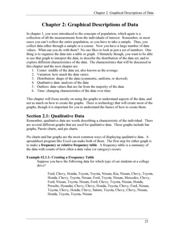
Chapter 2: Graphical Descriptions of DataGraph #2.2.1: Histogram for Monthly Rent402Frequency68Monthly Rent Paid by Students5001000150020002500Monthly Rent ( )If no frequency distribution was created before the histogram, then the commandwould be:hist(variable, col "type in what color you want", number of classes,main "type the title you want", xlab "type the label you want for thehorizontal axis") – produces histogram with specified color and number ofclasses (though the number of classes is an estimate and R will create thenumber of classes near this value).For this example, the R command without a frequency distribution created firstwould be:hist(rent, col "blue", 7, main "Monthly Rent Paid by Students",xlab "Monthly Rent ( )")Notice the graph has the axes labeled, the tick marks are labeled on each axis, andthere is a title.Reviewing the graph you can see that most of the students pay around 750 permonth for rent, with about 1500 being the other common value. You can seefrom the graph, that most students pay between 600 and 1600 per month forrent. Of course, these values are just estimates from the graph. There is a large42

Chapter 2: Graphical Descriptions of Datagap between the 1500 class and the highest data value. This seems to say thatone student is paying a great deal more than everyone else. This value could beconsidered an outlier. An outlier is a data value that is far from the rest of thevalues. It may be an unusual value or a mistake. It is a data value that should beinvestigated. In this case, the student lives in a very expensive part of town, thusthe value is not a mistake, and is just very unusual. There are other aspects thatcan be discussed, but first some other concepts need to be introduced.Frequencies are helpful, but understanding the relative size each class is to the total isalso useful. To find this you can divide the frequency by the total to create a relativefrequency. If you have the relative frequencies for all of the classes, then you have arelative frequency distribution.Relative Frequency DistributionA variation on a frequency distribution is a relative frequency distribution. Instead ofgiving the frequencies for each class, the relative frequencies are calculated.frequencyRelative frequency # of data pointsThis gives you percentages of data that fall in each class.Example #2.2.3: Creating a Relative Frequency TableFind the relative frequency for the grade data.Solution:From example #2.2.1, the frequency distribution is reproduced in table #2.2.2.Table #2.2.2: Frequency Distribution for Monthly RentClass Limits350 – 664665 – 979980 – 12941295 – 16091610 – 19241925 – 22392240 – 2554ClassClassBoundariesMidpoint Frequency349.5 – 664.55074664.5 – 979.58228979.5 – 1294.5113751294.5 – 1609.5 145261609.5 – 1924.5 176701924.5 – 2239.5 208202239.5 – 2554.5 23971Divide each frequency by the number of data points.485 0.17, 0.33, 0.21, 24242443

Chapter 2: Graphical Descriptions of DataTable #2.2.3: Relative Frequency Distribution for Monthly RentClassClassRelativeClass LimitsBoundariesMidpoint Frequency Frequency350 – 664349.5 – 664.550740.17665 – 979664.5 – 979.582280.33980 – 1294 979.5 – 1294.5113750.211295 – 1609 1294.5 – 1609.5 145260.251610 – 1924 1609.5 – 1924.5 1767001925 – 2239 1924.5 – 2239.5 2082002240 – 2554 2239.5 – 2554.5Total23971240.041The relative frequencies should add up to 1 or 100%. (This might be off a littledue to rounding errors.)The graph of the relative frequency is known as a relative frequency histogram. It looksidentical to the frequency histogram, but the vertical axis is relative frequency instead ofjust frequencies.Example #2.2.4: Drawing a Relative Frequency HistogramDraw a relative frequency histogram for the grade distribution from example#2.2.1.Solution:The class boundaries are plotted on the horizontal axis and the relativefrequencies are plotted on the vertical axis. (This is not easy to do in R, so useanother technology to graph a relative frequency histogram.)Graph #2.2.2: Relative Frequency Histogram for Monthly RentNotice the shape is the same as the frequency distribution.44

Chapter 2: Graphical Descriptions of DataAnother useful piece of information is how many data points fall below a particular classboundary. As an example, a teacher may want to know how many students receivedbelow an 80%, a doctor may want to know how many adults have cholesterol below 160,or a manager may want to know how many stores gross less than 2000 per day. This isknown as a cumulative frequency. If you want to know what percent of the data fallsbelow a certain class boundary, then this would be a cumulative relative frequency. Forcumulative frequencies you are finding how many data values fall below the upper classlimit.To create a cumulative frequency distribution, count the number of data points that arebelow the upper class boundary, starting with the first class and working up to the topclass. The last upper class boundary should have

spreadsheet program like Excel can make both of them. The first step for either graph is to make a frequency or relative frequency table. A frequency table is a summary of the data with counts of how often a data value (or category) occurs. Example #2.1.1: Creating a Frequency Table