Transcription
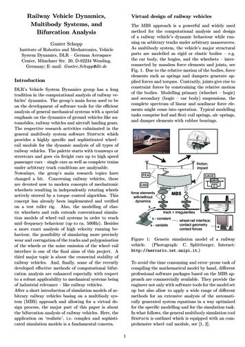
Railway Vehicle Dynamics,Multibody Systems, andBifurcation AnalysisVirtual design of railway vehiclesThe MBS approach is a powerful and widely usedmethod for the computational analysis and designof a railway vehicle’s dynamic behaviour while running on arbitrary tracks under arbitrary manoeuvres.As multibody system, the vehicle’s major structuralparts are modelled as rigid or elastic bodies – e.g.the car body, the bogies, and the wheelsets – interconnected by massless force elements and joints, seeFig. 1. Due to the relative motion of the bodies, forceelements such as springs and dampers generate applied forces and torques. Contrarily, joints give rise toconstraint forces by constraining the relative motionof the bodies. Modelling primary (wheelset – bogie)and secondary (bogie – car body) suspensions, thecomplete spectrum of linear and nonlinear force elements might come into operation. Typical modellingtasks comprise leaf and flexi–coil springs, air–springs,and damper elements with rubber bearings.Gunter SchuppInstitute of Robotics and Mechatronics, VehicleSystem Dynamics, DLR – German AerospaceCenter, Münchner Str. 20, D-82234 Wessling,Germany; E–mail: Gunter.Schupp@dlr.deIntroductionDLR’s Vehicle System Dynamics group has a longtradition in the computational analysis of railway vehicles’ dynamics. The group’s main focus used to beon the development of software tools for the efficientanalysis of general mechanical systems with a specialemphasis on the dynamics of ground vehicles like automobiles, railway vehicles and aircraft landing gears.The respective research activities culminated in thegeneral multibody system software Simpack whichprovides a highly specific and sophisticated wheel–rail module for the dynamic analysis of all types ofrailway vehicles. The palette starts with tramways orstreetcars and goes via freight cars up to high speedpassenger cars – single cars as well as complete trainsunder arbitrary track conditions are analysable.Nowadays, the group’s main research topics havechanged a bit. Concerning railway vehicles, theseare devoted now to modern concepts of mechatronicwheelsets resulting in independently rotating wheelsactively steered by a torque–control algorithm. Thisconcept has already been implemented and verifiedon a test roller rig. Also, the modelling of elastic wheelsets and rails extends conventional simulation models of wheel–rail systems in order to reachmid–frequency behaviour (up to ca. 500Hz). Besidesa more exact analysis of high velocity running behaviour, the possibility of simulating more preciselywear and corrugation of the tracks and polygonisationof the wheels or the noise emission of the wheel–railinterface is one of the final aims of this project. Athird major topic is about the crosswind stability ofrailway vehicles. And, finally, some of the recentlydeveloped effective methods of computational bifurcation analysis are enhanced especially with respectto a robust applicability to mechanical systems beingof industrial relevance – like railway vehicles.After a short introduction of simulation models of arbitrary railway vehicles basing on a multibody system (MBS) approach and allowing for a virtual design process, the major part of this paper is aboutthe bifurcation analysis of railway vehicles. Here, theapplication on ‘realistic’, i.e. complex and sophisticated simulation models is a fundamental concern.f r i ct i oi mFEpna,cACtACEMCf or cwdeei t h/ wynAl eDmei t hamBSCnot si cuMtBSsst r ass-vcaonr i asbt al ecnk i r r egtuwhccl aeoonnr i t i eel - r at at asccttgf oi li neomr cet er f aece:t r ysFigure 1: Generic simulation model of a railwayvehicle. (Photograph: C. Splittberger, Internet:http://mercurio.iet.unipi.it.)To avoid the time consuming and error–prone task ofcompiling the mathematical model by hand, differentprofessional software packages based on the MBS approach are commercially available. They provide theengineer not only with software tools for the model setup but also allow to apply a wide range of differentmethods for an extensive analysis of the automatically generated system equations in a way optimizedfor the specific modelling and for the simulation task.In what follows, the general multibody simulation toolSimpack is outlined which is equipped with an comprehensive wheel–rail module, see [1, 2].1
Concerning modern design concepts, certain simulation tasks and requirements may go beyond thescope of the typical MBS approach. In this case, bi–directional interfaces to established and widely–usedCAE (Computer Aided Engineering) software allowto reproduce specific phenomena or to follow particular design principles. In Fig. 1 the more importantof such interfaces are summarised, too.To accomplish the growing demand for a reductionof the total vehicle weight by applying lightweightstructures or within the realm of a comfort analysis, it might be necessary to take the structural flexibility of some particular vehicle components into account. This is done usually by means of an interface to FEA (Finite Element Analysis) software. Theprocedure is in principle that first a certain numberof mode shapes of the bodies to be modelled elastically are pre–calculated by the FEA software. Then,within the subsequent nonlinear multibody simulations, these mode shapes can be used to superimposethe rigid body motions with small elastic deformations.The interface to CAD (Computer Aided Design) software facilitates and accelerates the MBS setup whilereducing the risk of modelling errors by the possibility of integrating directly graphical as well as physicalCAD data into the MBS model.Active tilting technique is an example for the inclusion of electronically controlled elements into a railway vehicle. The necessary control algorithms aredesigned usually by means of suitable CACE (Computer Aided Control Engineering) tools such as MATLAB/Simulink. Efficient interfaces to those softwaretools allow an integrated design approach followingmechatronic principles.In contrary to the modelling elements described up tonow, one of the characteristics of a railway vehicle isits guidance along the track. A comprehensive vehicledesign requires the simulation of different manoeuvreson arbitrary tracks, usually with stochastic irregularities superimposed. These irregularities are taken either directly from measuring data or are defined as astochastic process via its power spectral density. Andfinally the usual assumption of the rails’ profiles beingconstant along the track has to be abandoned for thesimulation of vehicles running through a switch.The second characteristic of railway vehicles heavilyinfluencing their dynamic running behaviour is thecontact between steel wheel and steel rail with theirprofile cross sections being the decisive factor. Foradequate simulation results the strong nonlinearity ofthe contact geometry as well as of the contact mechanics has to be taken into account. To give an ideaof at least the geometric nonlinearities, figure 2 showsthe cross sections of the common wheel–rail profilecombination S1002/UIC60–ORE with the potentialpoints of contact being interconnected. To smooththe discontinuities inherent in the straight forwardrigid contact model revealed in this figure, too, aquasi–elastic contact model is introduced in [3]; thesmoothed wheel’s lateral location of the point of contact is an indispensable prerequisite for an efficientsimulation of railway vehicles.sQuasi - el ast i ccont actmsWheeSo1d00el:L2010UaI C60- OREaofc onigt aidc tc opnot ainc ttm[ modme]ld0- 3- 4n0- 2i lt iot r e- 1Rc aR02loQ0uc o0f l a- 1ngans i- et alac ts t icmod0- 5y :Leleat er a0l wheel s h5if t[ mm]Figure 2: Profile combination S1002/UIC60–ORE :Left: Cross–sections of wheel and rail incl. potentialpoints of contact. Right: Contact point location s̄ s̄(y); y is the lateral shift between wheel and rail.Bifurcation analysisA prominent feature of nonlinear dynamical systemsis the possible dependence of their long–time behaviour on the initial state. This means that oneand the same system may show a multiplicity ofquantitatively and qualitatively totally different behaviour patterns of its steady state, i.e. for systemtime t , even though all the system’s parameters remain unchanged. If possible transient processesare neglected, stationary, periodic, quasi–periodic,and/or chaotic behaviour has to be expected. A computer aided method for the examination of nonlinear dynamical systems with respect to the influenceof one or more system parameters on existence andshape of these potential behaviour patterns is numerical bifurcation analysis, see e.g. [4] for an extensivedescription. This analysis can be performed either bymeans of a simple parameter variation over time integrations or by means of the more sophisticated directmethod of path–following or continuation. The principle of path–following combines methods for the directcomputation of a system’s steady state (up to now, robust algorithms exist only for stationary and periodicsolutions) with the continuation of one–dimensionalcurves in higher dimensional spaces.A crucial aspect within the comprehensive computational design of a railway vehicle’s running dynamicsconcerns its long–time behaviour while running on anideally straight track. Starting from an (initial) disturbance, the vehicle’s motion relative to the track isevaluated after all transient activity has died away,i.e. only its steady state is regarded. Of particular2
interest is the influence of certain system parameterslike the vehicle’s velocity or the coefficient(s) of a suspension element.Varying for example the vehicle’s velocity v, a typicalscenario given as bifurcation diagram in figure 3 is asfollows: As long as the velocities are small or moderate every initial disturbance decays down to a stationary equilibrium rapidly. As soon as the so–calledcritical velocity is reached, the vehicle’s long–time behaviour changes abruptly and radically and an initialdisturbance may result in the so–called hunting orlimit cycle motion, a periodically oscillating motionof the complete vehicle relative to the track that hasto be avoided in everyday operations. Detailed analyses have shown, see e.g. [5], that there even exists avelocity range vnlin v vlin , where the final steadystate depends qualitatively on the initial disturbance.Thus, for one and the same velocity of this range justas a stationary steady state a periodic steady state(hunting) has to be expected as well. The velocity vlincharacterises a Hopf bifurcation, whereas for v vnlina saddle node bifurcation is found.addl ei f u- nr caod6et i onDirect computation of limit cycle solutionsUnder a theoretical as well as under an algorithmicperspective the direct calculation of periodic solutionsis by far the most difficult and costly part of every bifurcation analysis. For equations of motion given asan autonomous system of Ordinary Differential Equations (ODE), ẏ f (y), y Rn , the task can be formulated as a Boundary Value Problem (BVP) withthe initial time t0 0, the unknown initial statess : y(t0 ) and the also unknown period TP :. 03xst abl eper i odc. 0st ar i obdl ei cHopfbi f ur cat i ont abl est at i ovnanr yl i nvul i nnst abl est at i onvar yys. 06. 030[ me. 0- 6]np- 3. 0. 0mu0[ maym. 0- 3. 0- 6. 00. 02. 55t i m7. 0et[ s. 510ẏ f (y)(1)0 y(TP , s) s .(2)Described below is the Poincaré Map Method, a special kind of single shooting method implemented inthe software tool Path to solve such BVPs, see [9].A Poincaré plane of the equations of motion (1) is a(n 1)–dimensional hyperplane in the n–dimensionalstate space being transversal to the flow ϕ(t, s) of thesystem, see figure 4. Starting from a point s near aperiodic solution (i.e. near a closed trajectory in statespace) and being located on a suitable Poincaré planeΣ of (1), s Σ, the flow ϕ(t, s) will hit Σ for thefirst time in the same direction again after the returntime TR , ϕ(TR , s) Σ. Then, via the time discretePoincaré map P : s ϕ(TR , s), the residual mapQ(s) : s q withmb]sycontinuation and the direct computation of limit cycles of DAEs is addressed rather scarecly in literature,see [8] for a different approach. 0]Q(s) : P(s) s ϕ(TR , s) s , Q(s) : Σ Σ (3)Figure 3: Typical bifurcation diagram of a wheel–rail–system. The bifurcation parameter is the velocity valong the track, ymax is the maximum relative lateraldisplacement of a wheelset.can be defined. A fixed point sp of the Poincaré mapP(s) representing a periodic solution of system (1)results now as zero of this residual map:Q(sp ) ϕ(TP , sp ) sp 0 .Computational bifurcation analysis is an ideal software tool for examining this kind of dynamic behaviour. A more detailed description of a softwareenvironment for the continuation based bifurcationanalysis of arbitrary mechanical systems developedin recent years at DLR can be found in [6, 7]. There,a special emphasis is placed on the application on realistic and therefore necessarily complex simulationmodels of arbitrary railway vehicles. Algorithms andanalyses are restricted to stationary and periodic behaviour, i.e. to the range of technical–industrial relevance within railway vehicle dynamics. Three major topics are of primary interest: The integration ofthe bifurcation software Path into the software package Simpack for the simulation of general mechanicalsystems; the direct calculation of periodic solutions(limit cycles); and the handling of differential algebraic equations (DAEs). The following section concentrates on the second topic; the third topic, i.e. thejsyqswQ( s1P )yn( sj 2y)p3y( t , s(4)S)( TR, s)SSFigure 4: Poincaré plane, Poincaré map, and residualmap of a dynamical system’s flow ϕ(t, s) in R3 .One advantage of this method is that it can be enhanced on systems of DAEs f (ẏ, y) 0 via the concept of a reduced Poincaré map quite easily, see also[8] for a more detailed description.3
Thus, to compute a periodic solution directly, the system of nonlinear equations (4) has to be solved. Thisis done as usually by a Newton iteration of the typeQjs · sj Qj with the increment sj sj 1 sjand the Jacobian matrix Qs Q/ s. In principle,this gradient can be approximated column by columnvia finite differences; but for numerical reasons, asshown in [6] this approach leads easily to non–convergence of the iteration in case of larger or more complexMBS – like simulation models of complete railway vehicles taking into account the complete nonlinearitiesof the wheel–rail interface.As also proven and demonstrated in [6], a more reliable and more efficient way for the computation ofthe Jacobian Qs is to combine the outlined shootingmethod with an integrated sensitivity analysis of thesystem equations. The basic procedure is to generate the Jacobian Qs analytically on the base of thesensitivity matrix S(TR , s) : y(TR , s)/ s. On theother hand, differentiation of the initial value problem built from the system equations (1) and the initial condition y(t 0) s with respect to the unknown initial states s yields the Variational (Differential) Equations (VDE, with S(t, s) : y(t, s)/ s),Ṡ f ¡y(t, s) · S , yS(t0 0) I ,the integration of the nominal system. Then, compared to the former finite differences approach, theapproximation error of the Jacobian Qs is reducedfrom εQ O( TOL) down to εQ O(TOL) by thisalgorithm.Application on a passenger carFigure 5: Simulation model of an Avmz–passenger carwith Fiat 0270 bogies.The software environment for bifurcation analysis ofarbitrary mechanical systems mentioned above hasbeen applied on a couple of simulation models of railway vehicles showing different degrees of complexity.In what follows, some results of the bifurcation analyses performed for a 1st class Avmz coach’s modelgiven in figure 5 are presented. The modelling is according to the benchmark description [12]. The complexity of this model is typical for models used withinindustry for the extensive computational analysis anddesign of a railway vehicle’s running behaviour.The mechanical model of the passenger car consistsof altogether 15 rigid bodies. The suspension system comprises flexicoil springs with nearly paralleldampers, yaw and lateral dampers, as well as stifflateral bump stops. All the springs are modelledwith constant stiffness while each damper shows anonly piecewise linear (thus nonlinear) force–velocity–characteristic with a serial stiffness superimposed;hence, the eigendynamics of these damper elementshave to be considered, too. The state space of thevehicle model is described by altogether 114 position,velocity, and algebraic coordinates. Hence, a totalof 9576 equations has to be integrated for limit cycle calculations (i.e. the nominal system (1) and thevariational equations (5)).Some results of the respective bifurcation analysis aredisplayed in figure 6. The dynamic long–time behaviour of the vehicle depending on the velocity vas varied system parameter is represented in the bifurcation diagram to the left by the maximum lateraldeviation y of the leading wheelset with respect to thetrack. The stability of the limit cycle solutions can beevaluated by the evolution of the complex Floquet–multipliers (the eigenvalues of the monodromy matrix(5)a set of altogether n · n differential equations inthe unknown sensitivities Si,j : yi / sj , i, j 1, . . . , n. Consequently, besides solving the systemequations (1) (the nominal system) for the flow ϕ(t TR , s), this method requires the n2 VDEs (5) (the sensitivity system) to be solved for the sensitivity matrixS(t TR , s) additionally.The basic principle now is the synchronous integration of the nominal and the sensitivity system bymeans of the code Dagsl, see [6], a derivative ofthe famous DAE–solver Dassl, see [10]. Followingroughly the algorithm described in [11], in every single time step tm Dagsl first calculates the discretesolution ym of the nominal system (1) by a BDF–approach (BDF–Backward Differentiation Formula)and a modified Newton iteration as usually. Imqmediately after convergence of the iterates ym, then independent, discrete sensitivity vectors Si,m ym / si , i 1, . . . , n follow from an analogous BDF–discretisation of the variational equations (5) basingon the current solution (ym , ẏm ) in a subsequent, sequential (or parallel) loop. Due to the linearity of (5)this means merely the additional solution of n systems of linear equations. It must be emphasised thatthe VDEs do not have to be defined by the user (orthe surrounding MBS–algorithm generating the equations of motion) but are derived internally only ona purely numerical base by the Dagsl–algorithm itself. Let TOL be the error tolerances applied for4
M S(TP , sp )) given to the right of figure 6: A solution is stable if and only if the moduli of all thesemultipliers (besides one) are less than one.Floquet multiplierslateral shift of wheelset 1154 C 2Im(µ)max yWS 1 [mm]6321080A B100120 140v [m/s]160Though throughout the paper a particular emphasisis laid on wheel–rail systems, the software environment’s potential range of application is of course notrestricted to this specific case. Decoupled form theMBS–code, the bifurcation algorithms can be appliedon general dynamical systems just as well.1800.80.60.40.20 0.2 0.4 0.6 0.8 1References 0.50Re(µ)0.5[1] W. Rulka. Effiziente Simulation der Dynamikmechatronischer Systeme für industrielle Anwendungen. PhD thesis, Technical University of Vienna, Austria, 1998.1Figure 6: Bifurcation analysis of the Avmz passenger car. Left: Numerically computed bifurcation diagram. Right: Floquet–multipliers of the limit cyclesolutions.[2] G. Schupp and A. Jaschinski. Virtual Prototyping: The Future Way of Designing RailwayVehicles. Int. J. of Vehicle Design, 22(1/2):93–115, 1999.The stationary solutions are continued from nearlyzero velocity up to the first Hopf bifurcation A, characterised by the velocity vlin vA 101.62 m/s, andbeyond, where a second Hopf bifurcation B is detected. Up to now, it is not possible to continue theunstable limit cycle solutions branching off from Hopfbifurcation A. Therefore, the first step to continue periodic attractors is to generate an initial estimationwith the help of a conventional, external time integration. Here, this was done for a velocity v 130.0 m/s.For decreasing velocities, the path of stable periodicsolutions ends in the saddle–node bifurcation C atvnlin vC 95.62 m/s. This kind of bifurcation is indicated by the Floquet–multipliers with one of themcrossing the stability limit, i.e. the unit circle, alongthe real axis. Since below this limiting velocity no oscillations occur, it also represents the critical velocityfor this type of vehicle. For increasing velocities, theamplitude of the limit cycle oscillations grows ratherslowly due to the nonlinear geometry of wheel andrail profiles and the increasing intensity of the contact between the flanges of the wheels and the rails.[3] H. Netter. Rad–Schiene–Systeme in differential–algebraischer Darstellung. FortschrittsberichteVDI Reihe 12 Nr. 352. VDI Verlag, Düsseldorf,1998.[4] R. Seydel. Practical Bifurcation and StabilityAnalysis: From Equilibrium to Chaos. Springer–Verlag, New York, 1994.[5] H. True and J.C. Jensen. Parameter Study ofHunting and Chaos in Railway Vehicle Dynamics. In The Dynamics of Vehicles on Roads andTracks, 13th IAVSD–Symposium, 1993, pages508–521. Swets & Zeitlinger B.V., Lisse, 1993.[6] G. Schupp. Numerische Verzweigungsanalysemit Anwendungen auf Rad–Schiene–Systeme.Shaker Verlag, Aachen, 2004.[7] G. Schupp. Bifurcation Analysis of Railway Vehicles. Multibody System Dynamics, 2004. (to bepublished soon).[8] C. Franke and C. Führer. Collocation Methodsfor the Investigation of Peridic Motions of Constrained Multibody Systems. Multibody SystemDynamics, 5:133–158, 2001.ConclusionsThe paper gives a short overview of the MBS–modelling of general railway vehicles and the bifurcation analysis of the resulting simulation models. Described partially is a software environment for thecontinuation based bifurcation analysis of complexmechanical systems that has been developed at DLRin recent years. As a result of this software project,bifurcation analysis is now available as an additionalanalysis tool of a software package for the simulationof mechanical systems – including railway vehicles.The application on a passenger car’s ‘complete’ simulation model proves the applicability of the developed software on detailed, realistic and therefore necessarily complex models being of industrial relevance.[9] C. Kaas–Petersen. Chaos in a Railway Bogie.Acta Mechanica, 61:89–107, 1986.[10] K.E. Brenan, S.L. Campbell, and L.R. Petzold. Numerical Solution of Initial–Value Problems in Differential–Algebraic Equations. SIAM,Philadelphia, USA, 1996.[11] W.F. Feery, J.E. Tolsma, and P.I. Barton. Efficient Sensitivity Analysis of Large–Scale Differential–Algebraic Systems. Applied NumericalMathematics, 25:41–54, 1997.5
[12] Vehicle Data for 1st Class Avmz Coach with Fiat0270 Bogies (Appendix 1). In: ERRI B 176/DT290: B176/3 Benchmark Problem Results andAssessment. Utrecht, Holland, 1993.6
railway vehicles. The palette starts with tramways or streetcars and goes via freight cars up to high speed passenger cars - single cars as well as complete trains under arbitrary track conditions are analysable. Nowadays, the group's main research topics have changed a bit. Concerning railway vehicles, these