WIXLIB

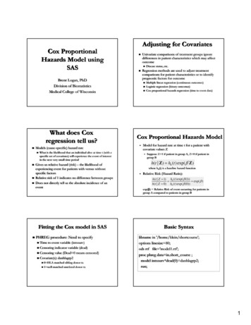
Cox ProportionalHazards Model usingSASAdjusting for Covariates Univariate comparisons of treatment groups ignoredifferences in patient characteristics which may affectoutcome Regressiongmethods are used to adjustj treatmentcomparisons for patient characteristics or to identifyprognostic factors for outcome Brent Logan, PhDDivision of BiostatisticsMedical College of WisconsinWhat does Coxregression tell us? Models (cause-specific) hazard rate Gives us relative hazard (risk) – the likelihood ofexperiencing event for patients with versus withoutspecific factorsRelative risk of 1 indicates no difference between groupsDoes not directly tell us the absolute incidence of aneventFitting the Cox model in SAS PHREG procedure: Need to specifyTime to event variable (intxsurv) Censoring indicator variable (dead) CensoringC n rin valuel (D(Dead 0d 0 meansm n censored)n r d) Covariate(s): danhlagrp2 0 HLA matched sibling donor tx1 well-matched unrelated donor txMultiple linear regression (continuous outcomes)Logistic regression (binary outcomes)Cox proportional hazards regression (time to event data)Cox Proportional Hazards Model What is the likelihood that an individual alive at time t (with aspecific set of covariates) will experience the event of interestin the next very small time period Disease status, etc.Model for hazard rate at time t for a patient withcovariate values Z Suppose Z 1 if patient in group A, Z 0 if patient ingroup Bh(t Z) h0 (t ) exp( β ' Z)where h0(t) is a baseline hazard function Relative Risk (Hazard Ratio):h(t Z 1) h0 (t ) exp( β (1)) exp( β )h(t Z 0) h0 (t ) exp( β (0))exp(β) Relative Risk of event occurring for patients ingroup A compared to patients in group BBasic Syntaxlibname in '/home/klein/shortcourse';options linesize 80;ods rtf file 'model1.rtf';proc phreg data in.short course ;model intxsurv*dead(0) danhlagrp2;run;1

Basic OutputBasic OutputDependent VariableCensoring Variable866866Number of Observations ReadNumber of Observations UsedModel InformationIN.SHORT COURSEData SetINTXSURVSummary of the Number of Event andCensored ValuesDEADCensoring Value(s)0Ties HandlingBRESLOWBasic .23Basic OutputConvergence StatusTesting Global Null Hypothesis: BETA 0Convergence criterion (GCONV 1E-8) satisfied.Lack of convergence indicates a problem with the modelTestLikelihood RatioModel Fit -2 LOG L6071.3686054.332AIC6071.3686056.33217.12861 .0001Wald16.92851 .0001These are 3 similar tests of whether the collective model(all variables) is better than no variables in the modelMain ResultObtaining Confidence IntervalsAnalysis of Maximum Likelihood rorChiSquare Pr ChiSq0.09150 16.9285DF Pr ChiSq1 .0001ScoreSBC6071.3686060.512Lower values indicate better fit. We will discuss more laterParameterEstimateChi-Square17.0360 .0001 Use risk limits option /rlHazardRatio1.457P-valueproc phreg data in.short course ;model intxsurv*dead(0) danhlagrp2 /rl ;run; Patients receiving well-matched unrelated donor transplants are1.457 times more likely to experience mortality at any time aftertransplant than patients receiving matched sibling donortransplants. This difference is statistically significant (p 0.0001).2

Obtaining Confidence IntervalsModelling continuous covariatesAnalysis of Maximum Likelihood ndardErrorChiSquarePr ChiSqHazardRatio10.376470.0915016.9285 .00011.45795% HazardRatioConfidenceLimits1.218 1.743 The hazard ratio for mortality for patients receivingwell-matched unrelated donor transplant vs. thosereceiving matched sibling donor transplant is 1.457,with a 95% confidence interval of [1.218-1.743]Checking the functional form Analysis of Maximum Likelihood 00079700.03276ChiSquare Pr ChiSq0.00060.9806HazardRatio1.00195% Hazard RatioConfidenceLimits0.939 Each increase in year of transplant is associated with a 1.001fold increase in risk of death (95% CI 0.939-1.067) This effect is not statistically significant (p 0.9806)1.067 Linearity of continuous covariate h(t Z) ho(t) exp[βg(Z)] What is the functional form of g(Z)?Plot of cumulative Martingaleg residuals againstglevels ofcovariate. Unusually large values suggest a problem with the functionalformASSESS statement in SAS includes Checking the functional formOne year increase in year of transplantproc phreg data in.short course ;model intxsurv*dead(0) yeartx/rl;run;Modelling continuous covariatesParameterYear of transplant can be modeled continuouslyExp(β) is interpreted as the hazard ratio orrelative risk associated with a one unit increasein covariate valueval ePlot of randomly generated residual processes to allow forgraphic assessment of the observed residuals in terms of whatis “too large”Formal hypothesis test based on simulationChecking the functional formproc phreg data in.short course ;model intxsurv*dead(0) yeartx/rl;v (y)/p ;assess var (yeartx)/resample;run;P-value No evidence of problems with linearity3

Categorical Covariates Categorical CovariatesSex: 1 Male, 2 FemaleConditioning Regimen (regimp): 1 NMA, 2 RIC,4 MYEPutting these variables into a model as continuouspredictorsdigivesiuninterpretableibl resultslSex could be recoded as an indicator variable (1 Male,0 Female)Conditioning Regimen could be recoded as multipleindicator variablesAutomatically implemented using CLASS statementproc phreg data in.short course ;class regimp;model intxsurvdead(0) regimp/rl;intxsurv*dead(0) regimp/rl;run;Categorical Covariates: OutputCategorical Covariates: OutputType 3 TestsClass Level InformationClassValueDesign Variablesregimp110201400EffectregimpCategorical Covariates: OutputParameter StandardEstimateErrorChiSquarePr ChiSqHazardRatioPr ChiSq0.0371Other pairwise comparisons Analysis of Maximum Likelihood EstimatesDFWaldChi-Square6.5865 Type 3 tests are an “overall” test of whether thereare any differences in event rate across any of thelevels of the covariate Here p 0.0371, indicating that there are significantdifferences in mortality between the threeconditioning regimens Doesn’t tell you which groups are different Sets up two indicator variables Z1 1 if regimp 1 (NMA) Z2 1 if regimp 2 (RIC) Baseline group is 4 (MA) Default baseline group is highest valueParameterDF295% HazardRatioConfidenceLimitsregimp110.381140 381140.149250 149256.52176 52170.01070 01071.4641 4641.0931 093 1.9611 961regimp210.080430.117370.46960.49321.0840.861 1.364 Default output tells you about hazard ratiosrelative to the baseline groupOther pairwise comparisons (e.g. RIC vs. NMAg) can be obtained throughgconditioning)Changing the baseline group/hazardratios option : Produces confidence intervalsfor RR for all pairwise comparisons Contrast statement: Hypothesis test for anycomparison of interest Hazard Ratios are interpreted relative to the baseline group (MA) Patients receiving NMA conditioning are 1.46 times more likely toexperience death at any time after tx than patients receiving MAregimens (p 0.0107) There is no significant difference in mortality between RICconditioning and MA conditioning (RR 1.08, p 0.4932)4

Changing the Baseline group Default baseline group is ref lastUse ref first to set the baseline group to the one with the lowestvalueproc phreg data in.short course ;class regimp (ref first);(ref first);model intxsurv*dead(0) regimp/rl;run;Global change to baseline group for all class variablesclass regimp /ref first;Can also specify a particular value for the baseline groupclass regimp (ref '1');Changing the Baseline groupAnalysis of Maximum Likelihood EstimatesParameterDFParameter StandardEstimateErrorChiSquare Pr ChiSqHazardRatio95% 3.00530.08300.7400.527 1.040regimp41-0.381140.149256.52170.01070.6830.510 0.915 Baseline group is now regimp 1 (NMA) Patients receiving RIC conditioning are 0.74 times as likely toexperience mortality at any time post transplant compared tothose receiving NMA regimens. This difference is not statistically significant (p 0.0830)HazardRatios optionHazardratios option: Outputproc phreg data in.short course ;class regimp;model intxsurv*dead(0) regimp/rl;( ) g phazardratios regimp;run;Hazard Ratios for regimpPointEstimateDescription95% WaldConfidenceLimitsregimp 1 vs 21.3510.9611.898regimp 1 vs 41.4641.0931.961regimp 2 vs 41.0840.8611.364Patients receiving NMA regimens are 1.351 times more likelyto experience mortality than patients receiving RICconditioning (95% CI 0.961-1.898)Contrast statement Contrast: Linear function of the β parametersC ci βi Interested in testingg the null hypothesisypthat thecontrast is equal to 0Z1 1 if NMA, 0 o/wZ2 1 if RIC, 0 o/wβ1 and β2 correspond to Z1 and Z2Hazard Ratio for NMA vs. RICh(t NMA) h0 (t ) exp( β1 ) exp( β1 β 2 )h(t RIC ) h0 (t ) exp( β 2 )Contrast Statement Testing whether the RR for NMA vs. RIC isequal to 1 is equivalent to testing H0:β1-β2 0Contrast coefficients (ci’s) are 1 and -1proc phreg data in.short course ;class regimp;model intxsurv*dead(0) regimp/rl;contrast ‘NMA vs. RIC' regimp 1 -1/estimate exp;run;5

Model AssumptionsContrast StatementContrast Test ResultsContrastDF1NMA vs. RICWaldChi-Square3.0053Pr ChiSq Cox model assumes that hazard ratios or relative risksare constant over time (proportional hazards) May be violated if one group has higher early risk ofdeath, while other group has higher late risk of death autotx vs. allotxllNeed to assess for each covariate whether thisassumption of proportional hazards is reasonableIf non-proportional hazards are present0.0830There is no statistically significant difference in mortality betweenNMA and RIC conditioning regimens (RR 1.351, 95%CI [0.9615-1.8978], p 0.0830) Contrast Rows Estimation and Testing Results ContrastTypeEXPNMA vs.RICRo Estimatwe11.3508StandardError 1.897 3.00538 Pr ChiSq0.0830 Assessing proportional hazards Assess statement in PROC PHREGPlot of standardized score residuals over time. Use separate relative risks for early and late (timedependent covariate approach)Stratified modelAssessing proportional hazards If the residuals get unusually large at any time point,this suggests a problem with the proportionalhazards assumptionCheck for non-proportional hazards withcovariate graftype (1 BM, 22 PB)proc phreg data in.short course ;class graftype;model intxsurv*dead(0) graftype/rl;assess ph/resample;run;SAS includesPlot of randomly generated score processes to allowfor graphic assessment of the observed residuals interms of what is “too large” Formal hypothesis test based on simulation Assessing proportional hazardsAssessing proportional hazards Observed score residual is too large relative torandomly generated sample processesP-value 0.021Thi iindicatesThisdiproportionali lhhazardsd assumptionidoes not hold when comparing BM vs. PBP-value6