Transcription
BetaCube: A Deep Reinforcement LearningApproach to Solving 2x2x2 Rubik’s Cubes WithoutHuman KnowledgeNicholas W. BowmanDepartment of Computer ScienceStanford UniversityStanford, CA 94305nbowman@stanford.eduJessica L. GuoDepartment of Computer ScienceStanford UniversityStanford, CA 94305jguo7@stanford.eduRobert M.J. JonesDepartment of Computer ScienceStanford UniversityStanford, CA 94305rmjones@stanford.eduAbstractAdvances in the field of deep reinforcement learning have led to the developmentof agents that can teach themselves how to solve problems in large, complexdomains without relying on any encoded human domain knowledge. The most wellknown of these agents was AlphaGo Zero, which was able to achieve superhumanperformance in the game of Go without any human supervision. Similar agentshave done well in games like Chess and Shogi. However, these games always haveguaranteed termination and a reward received at the end of the game, and oftencontain rewards throughout. By contrast, there are many interesting environments,such as combinatorial optimization problems, which involve sparse rewards andepisodes that are not guaranteed to terminate. One such task is finding a solution toa Rubik’s Cube, which has only one successful reward state and no guarantee ofepisode termination, since you can possibly continue making moves forever andnever achieve the solved state. In this paper we discuss our attempts to solve a2x2x2 cube (Mini Cube) using Autodidactic Iteration, a reinforcement learningalgorithm that is able to teach itself how to solve a cube without human guidance.In the end, given only the very basic physical rules that govern the evolution ofthe Rubik’s Cube as different moves are applied, our best model was able to solve100% of randomly scrambled cubes that were 4 moves away from the solved state.11.1IntroductionRubik’s CubeThe Rubik’s cube is a classic 3-Dimensional combination puzzle created in 1974 by inventor ErnoRubik. There are 6 faces which can be rotated 90 degrees in either direction in order to reach the goalstate of aligning all squares of the same color onto the same face of the cube. The Rubik’s cube has alarge state space, with approximately 4.3 1019 different possible configurations. However, out ofthis vast number of configurations, only one state is a goal state that presents a reward. Therefore,starting from random states and applying reinforcement learning algorithms could very likely resultin the agent never solving the cube and never receiving a learning signal.
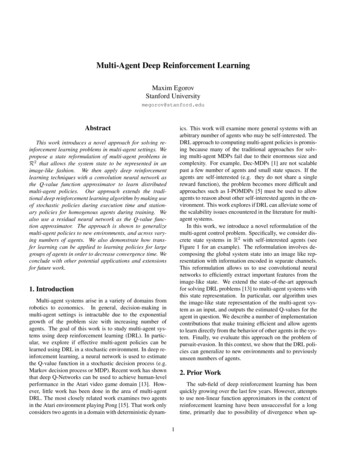
Given the limitations of the computational resources available to us, we chose to focus on solving aMini Cube for this investigation, which is simply a 2x2x2 Rubik’s cube. The Mini Cube consists of 8smaller cubes called cubelets, as opposed to the 26 cubelets in a traditional one. All cubelets in aMini Cube have 3 stickers attached to them, with 24 stickers in total. Because each sticker is uniquelyidentifiable based on the other stickers on the cubelet, we may use a one-hot encoding for each of the24 stickers to represent their location on the cube. We utilized the Py222 simulator framework [9] torepresent cubes and their evolving states when moves are applied.Moves on the cube are represented using face notation, which expresses which face to rotate with asingle letter. F, B, L, R, U, and D correspond to clockwise rotations of the front, back, left, right, up,and down faces respectively. The same letters followed by an apostrophe correspond to rotating thesame faces counterclockwise [10]. For a long time, there has been interest in the upper bound on thenumber of moves that is required to solve any scrambled Rubik’s cube, a number colloquially knownas God’s number. For a Mini Cube, this number has been proven to be 14 in the quarter turn metric,explained in [11].1.2Reinforcement LearningReinforcement learning (RL) is an area of machine learning where an agent learns how to behavein an environment by performing an action and seeing the rewards. Over the past several years, RLhas sparked interest, as it has been applied to a wide array of fields [5, 1, 2]. While RL has beensuccessful in many use cases, it depends on environments in which it can obtain informative rewardsas it takes a certain policy. In domains with very sparse rewards, RL algorithms do not perform nearlyas well [8]. Such domains include short answer exam problems, and combination puzzles such as theRubik’s Cube, which is why we were interested in exploring novel RL approaches to solving suchproblems.2Related WorkDeep Reinforcement Learning (DRL) broadly describes the use of deep neural networks to solveRL problems, and often involves training a model to predict the value function for a (state, action)pair [7]. Deep reinforcement learning techniques have been successful with such games as chessand Go [12, 13], and there have been recent efforts to use adapted versions of these techniques tosolve problems with sparser reward spaces. While many games have extremely large state spaces,the Rubik’s cube problem is unique because of its sparse reward space. The random turns of a cubeare difficult to evaluate as rewards because of the uncertainty in judging whether or not the newconfiguration is closer to a solution.Our work for this paper involved a modified implementation of McAleer et al.’s paper [8] that firstsolved the Rubik’s cube problem by augmenting a Monte Carlo Tree Search (MCTS) algorithmwith a trained neural network. MCTS is an online, heuristic search algorithm for decision makingprocesses that has enjoyed great success in game AI [4]. There are many variants of MCTS [3], twoof which we implement in this paper. It builds upon the ideas of Alpha Go Zero [14], whose neuralnetwork learns by generating its own training data (i.e., playing simulated games of Go against itself).3MethodsOur work was an attempt to recreate the methods outlined by McAleer et al.’s DeepCube paperwith a Mini Cube rather than a traditional 3x3x3 Rubik’s Cube. In addition to the original modelwe based off of DeepCube, we also trained three other neural networks with different sized layersand differently sized training sets to test their performance. We used each one of these models toaugment three different cube solving algorithms, two of which were Monte Carlo Tree Search-basedalgorithms.3.1TrainingTo train our network, we used autodidactic iteration (ADI), a supervised learning algorithm describedby McAleer et al. which trains a joint value and policy network [8]. In each training iteration, ADIstarts with a solved cube and makes random turns, using the resulting configurations as inputs for the2
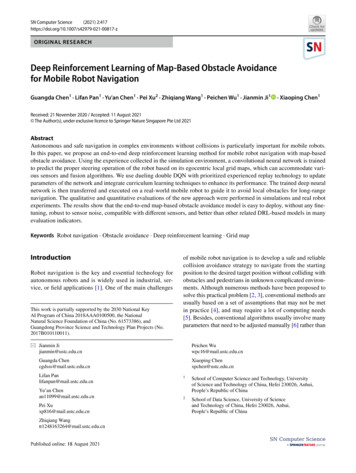
Figure 1: A visualization of ADI training set generationdeep neural network (DNN). Thus, the DNN has parameters θ, takes a state s as input, and outputs avalue-policy pair (v, p). The output policy, p, is a vector of probabilities of making each of the 12possible moves.We generated N k l training samples by starting with a solved cube, scrambling it k times tocreate a sequence of k cubes, and then repeating this process l different times. Targets were createdby performing a depth-1 breadth-first search from each training input state. For each of the childrenstates, we estimated the optimal value function by evaluating our current network. We calculated thevalue of each child as the DNN estimate plus the reward for that configuration, which was simply 1if it was a solved cube and -1 otherwise. We set the value target to be the maximal value of the set ofchildren, and similarly set the policy target to be the move that results in the maximal estimated value.Figure 1 provides a visual overview of the training set generation process for ADI, which is the keyinsight for developing a successful reinforcement learning algorithm in a problem state with suchsparse rewards. Algorithm 1 provides the pseudocode for this approach.Algorithm 1 Autodidactic Iteration1: procedure ADI2:Initialization: θ initialized using Glorot uniform inititalization3:repeat4:X N scrambled cubes5:for xi X do6:for a A do7:((vxi (a), pxi (a)) fθ (A(xi , a))8:yvi maxa (R(A(xi , a)) vxi (a))9:ypi argmaxa (R(A(xi , a)) vxi (a))10:Yi (yvi , ypi )11:θ0 train(fθ , X, Y )12:θ θ013:until iterations MThe structure of our neural network, fθ was the same as the one laid out in the DeepCube paper, whichused a feed forward network with the architecture shown in Figure 2. The input to the network is an8 24 matrix representing the one-hot encoding of the cube locations. The outputs of the networkare a 1 dimensional scalar v, representing the value, and a 12 dimensional vector p, representing theprobability of selecting each of the possible moves. Each adjacent layer was fully connected, andthe elu activation function was used on all of them except for the two output layers. We used theRMSProp optimizer for training, with mean squared error loss function for the value and softmax3
cross entropy loss for the policy. The network was then trained using ADI for a number of iterations.Our training machine was a 2 core Intel Xeon @ 2.20GHz with 1 Nvidia Tesla K80 GPU.We trained four different models using slightly different numbers for the training data and fθ sizes, as described in Table1. Model 1 trained with N 20 100 2000 samples for1000 iterations with the original architecture and size as in theMcAleer et al. paper [8]. This network witnessed approximately 4 million cubes, including repeats, and it trained fora period of 36 hours. Model 2 trained with N 20 100 2000 samples for 1000 iterations, but with all of the layers ofour network half the size as the original. Model 3 trained withN 25 200 5000 samples for 1000 iterations, with all ofthe layers of our network half the size as the original. Finally,Figure 2: Model ArchitectureModel 4 trained with N 25 100 2500 samples for 1200iterations, but with all of the layers of our network a quarterthe size as the original. The architecture of all models was the same, and the specific dimensionsof Models 2 and 3 are illustrated in Figure 2. All models were trained with an initial learning rateof η 0.0005. In Table 1, "full-sized" refers to a model matching the number and size of layerspresented in [8], and other model sizes are defined relative to this model.Table 1: Trained Neural Networks3.2ModelBatch SizeIterationsfθ SizeModel 1Model 2Model 3Model 420002000500025001000100010001200Full-sized layers12 -sized layers12 -sized layers14 -sized layersSolverOur baseline version of the solver, which we call Greedy, uses our trained probability vector networkas a heuristic in a greedy best-first search for a simple evaluation of the trained network. In theGreedy solver, we run our current cube state through the trained network and retrieve p and thenselect the move associated with the largest value in p.The second version of our solver, which we call Vanilla MCTS, uses our trained value and probabilityvector network to augment the MCTS algorithm described on page 102 of Decision Making UnderUncertainty [6]. Here, we use the value returned by the network as the Q0 initialization when weexpand to a previously unseen state. In addition, for the rollout policy we use a softmax explorationpolicy, utilizing the transition probabilities produced by our network for any given state. In our finalimplementation, we used λ 1 for this softmax exploration policy.The final version of our solver, which we refer to as Full MCTS, is again derived from the approachdescribed in the McAleer et al. paper [8]. In this algorithm, we build a search tree iteratively bybeginning with a tree consisting only of our starting state, T s0 . We then perform simulatedtraversals until reaching a leaf node of T . Each state, s T , has a memory attached to it storing:Ns (a), the number of times an action a has been taken from state s; Ws (a), the maximal valueof action a from state s; Ls (a), the current virtual loss for action a from state s; and Ps (a), theprior probability of action a from state s. The search strategy is defined by taking the actionP00 Nst (a )At defined by At argmaxa Ust (a) Qst (a), where Ust (a) c · Pst (a) Nsa (a) 1andtQst (a) Wst (a) Lst (a), until an unexpanded leaf node sτ is reached. Upon reaching anunexpanded node, we add the children of sτ to the tree T and initialize the weights for each childto be Ws0 (·) 0, Ns0 (·) 0, Ps0 (·) ps0 , and Ls0 (·) 0, where ps0 is the output of the policynetwork for s0 . Finally, we evaluate the neural network on state sτ to get vsτ and then back thisvalue up to all previously visited states by updating Wst (At ) max(Wst (At ), vsτ ) for all precedingnodes in our current tree traversal. The tree traversal process continues until we reach the goal solvedstate or reached a fixed number of computations.4
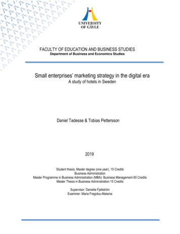
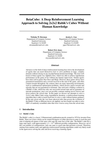
Figure 3: Comparison of solve rates across different solvers and trained neural networks4ResultsIn our analysis, we compared the three versions of the BetaCube solver described in the previoussection with the four different neural nets. In our testing, we ran the solver from zero to seven randomturns away from a solved cube for 50 times at each distance. We then took the percentage of cubesthat were solved in those 50 iterations as our points of comparison, and plotted our results, as seen inFigure 3.We first looked at how each of our neural net models compared to each other across all three solvers.Our Model 2, which saw approximately 4 million cubes and used a neural network with layers halfthe size as described in DeepCube, consistently performed the best. It was the only model which didnot see immediate steep drop offs for cubes that were one turn away from a solved state, and was theonly model which was able to solve cubes when used with Vanilla MCTS. Our Model 1, which sawthe same number of cubes, and used the same NN size as in DeepCube was neither the worst, nor thebest, and its performance depended on which algorithm it was implemented with. Knowing that ourModel 3 had the same NN as Model 2 and saw more training data, we expected it to perform better.However, this was not the case, and both Model 3 as well as Model 4, which trained with a very smallNN, both performed poorly regardless of the solver that was used. Possible explanations for this aredue to overfitting, or a NN that was too small, which we discuss in our conclusion. It should be notedthat in the second chart of Figure 3, Models 1, 3, and 4 all failed to solve any cubes that were greaterthan 0 steps away, and are plotted one on top of the other.We then moved on to the original focus of our paper, whichwas an implementation and evaluation of the Full MCTS algorithm as described in McAleer et al. [8] The Full MCTS andGreedy baseline algorithm worked similarly, with only resultsfrom Model 1 in Full MCTS underperforming compared to itsGreedy counterpart. While we expected the opposite result,this may be because MCTS works better for stochastic settings,whereas these configurations which are a very small numberof steps away would be better solved with a deterministic approach. We also implemented a Vanilla MCTS as another pointof reference to compare our Full MCTS to. While we expectedVanilla MCTS to perform somewhere in between the Greedysolver and Full MCTS, three out of four of our models failed Figure 4: Example of cube five stepsto solve any cubes with this algorithm. Interestingly, our best from solved stateperformance for any combination of models and solvers alsocame out of Vanilla MCTS, paired with Model 2. This combination was able to solve 100% of cubesfour moves away or less, and 75% of cubes five moves away, which include nontrivial cubes such asin Figure 4 that are difficult for the average person to solve. Given that none of the the three of uswere able to solve the pictured cube by hand, we were impressed by the algorithm’s ability to solve5
such cubes. Compared to DeepCube, however, which was able to solve more than 90% of 3x3x3cubes that were within 20 moves of the goal state, our best implementation still fell short of that levelof success.5ConclusionThere are a number of fixes and adjustments we propose for future work to address the shortcomingsof our implementation.5.1Network ArchitectureGiven the poor performance of Model 1 (defined in Table 1), we have reason to believe that theoriginal network from [8] was too complex for our problem, and that we were overfitting on ourtraining set. Future work would involve pursuing smaller network architectures, which includesboth decreasing the number of parameters per layer as well as possibly removing layers altogether.However, as witnessed by the poor performance of Model 4, making the number of parameters perlayer too small does not allow for sufficient expressivitiy to capture the nuances of the value functionand also leads to poor performance.5.2Training ProcessMcAleer et al. do not specify their findings about the relationship between N , the batch size of cubeson which the network trains, and M , the number of overall iterations to run ADI. For example, anetwork could see the same number of cubes (e.g., 2 million), with different values for N and M (e.g.,N 2000 and M 1000 v.s. N 100 and M 20000, etc.). These values are hyperparameters,and must be carefully tuned as with any machine learning process. Given the limited time andresources we had available to us, we were only able to choose a couple combinations of values totrain our neural networks.Additionally, having more computing power would be essential for iterating through different modelarchitectures and hyperparameters. With our Google Cloud setup, we were limited to training ona far smaller number of cubes compared to [8] (2 million cubes vs 8 billion cubes). Being ableto experiment with more models and larger training sets would better allow us to find the optimalnetwork for our problem.5.3MCTSOne immediate modification to our use of MCTS would be to increase the maximumdepth/computation time. In [8], McAleer et al. allow for a maximum runtime of 60 minutesfor their MCTS algorithm to find the solution state, whereas we capped our computation time at aminute in order to evaluate our algorithm on more cubes.A more ambitious improvement would be to implement a multi-threaded version of this MCTSalgorithm. In the asynchronous form, multiple worker threads could simultaneously explore differentpaths and stop once a solution is found. This would help to explore more potential paths down thetree and decrease the time necessary to navigate to the solved state.Finally, MCTS also has hyperparameters that require tuning. We found some success using theexploration parameter c equal to that of Alpha Go Zero (c 4), but a more robust solution wouldrequire experimenting with different values and optimizing over this hyperparameter.AcknowledgmentsWe would like to thank Jeremy Morton for providing the encouragement to explore implementationof the ideas presented in the McAleer et al. paper and the suggestion to experiment with smallerneural network sizes. We would also like to thank Shushman and Mykel for their advice during officehours.6
6Group ContributionsAll code used for this project and discussed in this section can be found on Github athttps://github.com/robbiejones96/RubiksSolver1. Nick focused on development of the three solver algorithms described in section 3.2. Heimplemented the greedy search algorithm, vanilla MCTS algorithm as described in textbooksection 4.6, and the full MCTS algorithm described in the McAleer et al. paper, all of whichare located in the MCTS.py file, along with some test harness code. He also developed someof the command line infrastructure present in the ADI.py file, which allowed for modelsaving/restoration and specification of which search algorithms to use.2. Robbie implemented the ADI algorithm by utilizing the py222 library and building themultitask neural network in Keras. He also setup the Google cloud architecture to train thedifferent models.3. Jessica helped with building the architecture of the neural network model that was used fortraining. She also worked with analysis portion of the project, comparing the results fromtesting run with each of the different [9][10][11][12][13][14]Pieter Abbeel et al. “An application of reinforcement learning to aerobatic helicopter flight”.In: Advances in neural information processing systems. 2007, pp. 1–8.Justin A Boyan and Michael L Littman. “Packet routing in dynamically changing networks:A reinforcement learning approach”. In: Advances in neural information processing systems.1994, pp. 671–678.Cameron Browne et al. “A Survey of Monte Carlo Tree Search Methods”. In: IEEE Transactions on Computational Intelligence and AI in Games 4:1 (Mar. 2012), pp. 1–43. DOI:10.1109/TCIAIG.2012.2186810.Guillaume Chaslot et al. “Monte-Carlo Tree Search: A New Framework for Game AI.” In:2008.Jens Kober and Jan Peters. “Reinforcement learning in robotics: A survey”. In: ReinforcementLearning. Springer, 2012, pp. 579–610.Mykel J. Kochenderfer et al. Decision Making Under Uncertainty: Theory and Application.1st. The MIT Press, 2015. ISBN: 9780262029254.Yuxi Li. “Deep Reinforcement Learning”. In: CoRR abs/1810.06339 (2018).Stephen McAleer et al. “Solving the Rubik’s Cube Without Human Knowledge”. In: CoRRabs/1805.07470 (2018). arXiv: 1805.07470. URL: http://arxiv.org/abs/1805.07470.MeepMoop. MeepMoop/py222. Oct. 2017. URL: https://github.com/MeepMoop/py222.Rubik’s Cube Notation. URL: https://ruwix.com/the-rubiks-cube/notation/.Jaap Scherphuis. Jaap’s Puzzle Page. URL: https://www.jaapsch.net/puzzles/cube2.htm.David Silver et al. “Mastering Chess and Shogi by Self-Play with a General ReinforcementLearning Algorithm”. In: CoRR abs/1712.01815 (2017).David Silver et al. “Mastering the game of Go with deep neural networks and tree search”. In:nature 529.7587 (2016), p. 484.David Silver et al. “Mastering the game of Go without human knowledge”. In: Nature 550(2017), pp. 354–359.7
2x2x2 cube (Mini Cube) using Autodidactic Iteration, a reinforcement learning algorithm that is able to teach itself how to solve a cube without human guidance. In the end, given only the very basic physical rules that govern the evolution of the Rubik's Cube as different moves are applied, our best model was able to solve