WIXLIB

Examples that are similar to each other (i.e. examples with similar attributevalues) tend to be assigned to the same cluster, whereas examples different fromeach other tend to be assigned to distinct clusters. Note that, once the clusters arefound, each cluster can be considered as a “class”, so that now we can run aclassification algorithm on the clustered data, by using the cluster name as a classlabel. GAs for clustering are discussed e.g. in [50], [17], [33].2.2.4 Discovery of Association Rules. In the standard form of this task (ignoringvariations proposed in the literature) each data instance (or “record”) consists of aset of binary attributes called items. Each instance usually corresponds to acustomer transaction, where a given item has a true or false value depending onwhether or not the corresponding customer bought that item in that transaction.An association rule is a relationship of the form IF X THEN Y, where X and Y aresets of items and X Y [1], [2]. An example is the association rule:IF fried potatoes THEN soft drink, ketchup .Although both classification and association rules have an IF-THEN structure,there are important differences between them. We briefly mention here two ofthese differences. First, association rules can have more than one item in the ruleconsequent, whereas classification rules always have one attribute (the goal one)in the consequent. Second, unlike the association task, the classification task isasymmetric with respect to the predicting attributes and the goal attribute.Predicting attributes can occur only in the rule antecedent, whereas the goalattribute occurs only in the rule consequent. A more detailed discussion about thedifferences between classification and association rules can be found in [24].2.3 The Knowledge Discovery ProcessThe application of a data mining algorithm to a data set can be considered thecore step of a broader process, often called the knowledge discovery process [18].In addition to the data mining step itself, this process also includes several othersteps. For the sake of simplicity, these additional steps can be roughly categorizedinto data preprocessing and discovered-knowledge postprocessing.We use the term data preprocessing in a general sense, including thefollowing steps (among others) [55]:(a) Data Integration - This is necessary if the data to be mined comes fromseveral different sources, such as several departments of an organization. Thisstep involves, for instance, removing inconsistencies in attribute names orattribute value names between data sets of different sources.(b) Data Cleaning - It is important to make sure that the data to be mined is asaccurate as possible. This step may involve detecting and correcting errors in thedata, filling in missing values, etc. Data cleaning has a strong overlap with dataintegration, if this latter is also performed. It is often desirable to involve the userin data cleaning and data integration, so that (s)he can bring her/his background

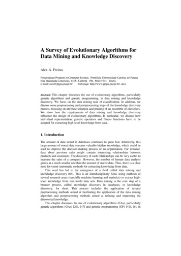
knowledge into these tasks. Some data cleaning methods for data mining arediscussed in [32], [59].(c) Discretization - This step consists of transforming a continuous attribute into acategorical (or nominal) attribute, taking on only a few discrete values - e.g., thereal-valued attribute Salary can be discretized to take on only three values, say“low”, “medium”, and “high”. This step is particularly required when the datamining algorithm cannot cope with continuous attributes. In addition,discretization often improves the comprehensibility of the discovered knowledge[11], [52].(d) Attribute Selection - This step consists of selecting a subset of attributesrelevant for classification, among all original attributes. It will be discussed insubsection 2.3.1.Discovered-knowledge postprocessing usually aims at improving thecomprehensibility and/or the interestingness of the knowledge to be shown to theuser. This step may involve, for instance, the selection of the most interestingrules, among the discovered rule set. This step will be discussed in subsection2.3.2.Note that the knowledge discovery process is inherently iterative, asillustrated in Fig. 1. As can be seen in this figure, the output of a step can be notonly sent to the next step in the process, but also sent – as a feedback - to aprevious step.input data.integrationpreproc.dataminingpostproc.input dataoutputknowledgeFig. 1. An overview of the knowledge discovery process2.3.1 Attribute Selection. This consists of selecting, among all the attributes ofthe data set, a subset of attributes relevant for the target data mining task. Notethat a number of data mining algorithms, particularly rule induction ones, alreadyperform a kind of attribute selection when they discover a rule containing just afew attributes, rather than all attributes. However, in this section we are interestedin attribute selection as a preprocessing step for the data mining algorithm.

Hence, we first select an attribute subset and then give only the selected attributesfor the data mining algorithm.The motivation for this kind of preprocessing is the fact that irrelevantattributes can somehow “confuse” the data mining algorithm, leading to thediscovery of inaccurate or useless knowledge [38]. Considering an extremeexample, suppose we try to predict whether the credit of a customer is good orbad, and suppose that the data set includes the attribute Customer Name. A datamining algorithm might discover too specific rules of the form:IF (Customer Name “a specific name”) THEN (Credit “good”). This kindof rule has no predictive power. Most likely, it covers a single customer andcannot be generalized to other customers. Technically speaking, it is overfittingthe data. To avoid this problem, the attribute Customer Name (and otherattributes having a unique value for each training example) should be removed ina preprocessing step.Attribute selection methods can be divided into filter and wrapper approaches.In the filter approach the attribute selection method is independent of the datamining algorithm to be applied to the selected attributes.By contrast, in the wrapper approach the attribute selection method uses theresult of the data mining algorithm to determine how good a given attributesubset is. In essence, the attribute selection method iteratively generates attributesubsets (candidate solutions) and evaluates their qualities, until a terminationcriterion is satisfied. The attribute-subset generation procedure can be virtuallyany search method. The major characteristic of the wrapper approach is that thequality of an attribute subset is directly measured by the performance of the datamining algorithm applied to that attribute subset.The wrapper approach tends to be more effective than the filter one, since theselected attributes are “optimized” for the data mining algorithm. However, thewrapper approach tends to be much slower than the filter approach, since in theformer a full data mining algorithm is applied to each attribute subset consideredby the search. In addition, if we want to apply several data mining algorithms tothe data, the wrapper approach becomes even more computationally expensive,since we need to run the wrapper procedure once for each data mining algorithm.2.3.2 Discovered-Knowledge Postprocessing. It is often the case that theknowledge discovered by a data mining algorithm needs to undergo some kind ofpostprocessing. Since in this chapter we focus on discovered knowledgeexpressed as IF-THEN prediction rules, we are mainly interested in thepostprocessing of a discovered rule set.There are two main motivations for such postprocessing. First, when thediscovered rule set is large, we often want to simplify it - i.e., to remove somerules and/or rule conditions - in order to improve knowledge comprehensibilityfor the user.Second, we often want to extract a subset of interesting rules, among alldiscovered ones. The reason is that although many data mining algorithms were

designed to discover accurate, comprehensible rules, most of these algorithmswere not designed to discover interesting rules, which is a rather more difficultand ambitious goal, as mentioned in section 2.1.Methods for selection of interesting rules can be roughly divided intosubjective and objective methods. Subjective methods are user-driven anddomain-dependent. For instance, the user may specify rule templates, indicatingwhich combination of attributes must occur in the rule for it to be consideredinteresting - this approach has been used mainly in the context of associationrules [40]. As another example of a subjective method, the user can give thesystem a general, high-level description of his/her previous knowledge about thedomain, so that the system can select only the discovered rules which representpreviously-unknown knowledge for the user [44].By contrast, objective methods are data-driven and domain-independent.Some of these methods are based on the idea of comparing a discovered ruleagainst other rules, rather than against the user’s beliefs. In this case the basicidea is that the interestingness of a rule depends not only on the quality of the ruleitself, but also on its similarity to other rules. Some objective measures of ruleinterestingness are discussed in [26], [22], [23].We believe that ideally a combination of subjective and objective approachesshould be used to try to solve the very hard problem of returning interestingknowledge to the user.3. Genetic Algorithms (GAs) for Rule DiscoveryIn general the main motivation for using GAs in the discovery of high-levelprediction rules is that they perform a global search and cope better with attributeinteraction than the greedy rule induction algorithms often used in data mining[14].In this section we discuss several aspects of GAs for rule discovery. Thissection is divided into three parts. Subsection 3.1 discusses how one can designan individual to represent prediction (IF-THEN) rules. Subsection 3.2 discusseshow genetic operators can be adapted to handle individuals representing rules.Section 3.3 discusses some issues involved in the design of fitness functions forrule discovery.3.1 Individual Representation3.1.1 Michigan versus Pittsburgh Approach. Genetic algorithms (GAs) for rulediscovery can be divided into two broad approaches, based on how rules areencoded in the population of individuals (“chromosomes”). In the Michiganapproach each individual encodes a single prediction rule, whereas in thePittsburgh approach each individual encodes a set of prediction rules.It should be noted that some authors use the term “Michigan approach” in a

narrow sense, to refer only to classifier systems [35], where rule interaction istaken into account by a specific kind of credit assignment method. However, weuse the term “Michigan approach” in a broader sense, to denote any approachwhere each GA individual encodes a single prediction rule.The choice between these two approaches strongly depends on which kind ofrule we want to discover. This is related to which kind of data mining task we areaddressing. Suppose the task is classification. Then we usually evaluate thequality of the rule set as a whole, rather than the quality of a single rule. In otherwords, the interaction among the rules is important. In this case, the Pittsburghapproach seems more natural.On the other hand, the Michigan approach might be more natural in otherkinds of data mining tasks. An example is a task where the goal is to find a smallset of high-quality prediction rules, and each rule is often evaluated independentlyof other rules [49]. Another example is the task of detecting rare events [65].Turning back to classification, which is the focus of this chapter, in a nutshellthe pros and cons of each approach are as follows. The Pittsburgh approachdirectly takes into account rule interaction when computing the fitness function ofan individual. However, this approach leads to syntactically-longer individuals,which tends to make fitness computation more computationally expensive. Inaddition, it may require some modifications to standard genetic operators to copewith relatively complex individuals. Examples of GAs for classification whichfollow the Pittsburgh approach are GABIL [13], GIL [37], and HDPDCS [51].By contrast, in the Michigan approach the individuals are simpler andsyntactically shorter. This tends to reduce the time taken to compute the fitnessfunction and to simplify the design of genetic operators. However, this advantagecomes with a cost. First of all, since the fitness function evaluates the quality ofeach rule separately, now it is not easy to compute the quality of the rule set as awhole - i.e. taking rule interactions into account. Another problem is that, sincewe want to discover a set of rules, rather than a single rule, we cannot allow theGA population to converge to a single individual - which is what usually happensin standard GAs. This introduces the need for some kind of niching method [45],which obviously is not necessary in the case of the Pittsburgh approach. We canavoid the need for niching in the Michigan approach by running the GA severaltimes, each time discovering a different rule. The drawback of this approach isthat it tends to be computationally expensive. Examples of GAs for classificationwhich follow the Michigan approach are COGIN [30] and REGAL [28].So far we have seen that an individual of a GA can represent a single rule orseveral rules, but we have not said yet how the rule(s) is(are) encoded in thegenome of the individual. We now turn to this issue. To follow our discussion,assume that a rule has the form “IF cond1 AND . AND condn THEN class ci “,where cond1 . condn are attribute-value conditions (e.g. Sex “M”) and ci is theclass predicted by the rule. We divide our discussion into two parts, therepresentation of the rule antecedent (the “IF” part of the rule) and therepresentation of the rule consequent (the “THEN” part of the rule). These two

issues are discussed in the next two subsections. In these subsections we willassume that the GA follows the Michigan approach, to simplify our discussion.However, most of the ideas in these two subsections can be adapted to thePittsburgh approach as well.3.1.2 Representing the Rule Antecedent (a Conjunction of Conditions). Asimple approach to encode rule conditions into an individual is to use a binaryencoding. Suppose that a given attribute can take on k discrete values. Then wecan encode a condition on the value of this attribute by using k bits. The i-th value(i 1,.,k) of the attribute domain is part of the rule condition if and only if thei-th bit is “on” [13].For instance, suppose that a given individual represents a rule antecedent witha single attribute-value condition, where the attribute is Marital Status and itsvalues can be “single”, “married”, “divorced” and “widow”. Then a conditioninvolving this attribute would be encoded in the genome by four bits. If these bitstake on, say, the values “0 1 1 0” then they would be representing the followingrule antecedent:IF (Marital Status “married” OR “divorced”)Hence, this encoding scheme allows the representation of conditions withinternal disjunctions, i.e. with the logical OR operator within a condition.Obviously, this encoding scheme can be easily extended to represent ruleantecedents with several conditions (linked by a logical AND) by including in thegenome an appropriate number of bits to represent each attribute-value condition.Note that if all the k bits of a given rule condition are “on”, this means that thecorresponding attribute is effectively being ignored by the rule antecedent, sinceany value of the attribute satisfies the corresponding rule condition. In practice, itis desirable to favor rules where some conditions are “turned off” - i.e. have alltheir bits set to “1” – in order to reduce the size of the rule antecedent. (Recallthat we want comprehensible rules and, in general, the shorter the rule is the morecomprehensible it is.) To achieve this, one can automatically set all bits of acondition to “1” whenever more than half of those bits are currently set to “1”.Another technique to achieve the same effect will be discussed at the end of thissubsection.The above discussion assumed that the attributes were categorical, also callednominal or discrete. In the case of continuous attributes the binary encodingmechanism gets slightly more complex. A common approach is to use bits torepresent the value of a continuous attribute in binary notation. For instance, thebinary string “0 0 0 0 1 1 0 1” represents the value 13 of a given integer-valuedattribute.Instead of using a binary representation for the genome of an individual, thisgenome can be expressed in a higher-level representation which directly encodesthe rule conditions. One of the advantages of this representation is that it leads toa more uniform treatment of categorical and continuous attributes, in comparison

with the binary representation.In any case, in rule discovery we usually need to use variable-lengthindividuals, since, in principle, we do not know a priori how many conditions willbe necessary to produce a good rule. Therefore, we might have to modifycrossover to be able to cope with variable-length individuals in such a way thatonly valid individuals are produced by this operator.For instance, suppose that we use a high-level representation for twoindividuals to be mated, as follows (there is an implicit logical AND connectingthe rule conditions within each individual):(Age 25) (Marital Status “Married”)(Has a job “yes”) (Age 21)As a result of a crossover operation, one of the children might be an invalidindividual (i.e. a rule with contradicting conditions), such as the following ruleantecedent:IF (Age 25) AND (Age 21).To avoid this, we can modify the individual representation to encode attributes inthe same order that they occur in the data set, including in the representation“empty conditions” as necessary. Continuing the above example, and assumingthat the data set being mined has only the attributes Age, Marital Status, andHas a job, in this order, the two above individuals would be encoded as follows:(Age 25) (Marital Status “married”) (“empty conditon”)(Age 21) (“empty condition”)(Has a job “yes”)Now each attribute occupies the same position in the two individuals, i.e.attributes are aligned [21]. Hence, crossover will produce only valid individuals.This example raises the question of how to determine, for each gene, whetherit represents a normally-expressed condition or an empty condition. A simpletechnique for solving this problem is as follows. Suppose the data being minedcontains m attributes. Then each individual contains m genes, each of themdivided into two parts. The first one specifies the rule condition itself (e.g. Age 25), whereas the second one is a single bit. If this bit is “on” (“off”) the conditionis included in (excluded from) the rule antecedent represented by the individual.In other w

data mining and knowledge discovery. We focus on the data mining task of classification, which is the task addressed by most EAs that extract high-level knowledge from data. In addition, we discuss the use of EAs for performing some preprocessing and postprocessing steps of the knowledge discovery process,