Transcription
Synbols: Probing Learning Algorithms withSynthetic DatasetsAlexandre Lacoste1 , Pau Rodríguez1 , Frédéric Branchaud-Charron1 , Parmida Atighehchian1 ,Massimo Caccia1,2 , Issam Laradji1 , Alexandre Drouin1 , Matt Craddock1 , Laurent Charlin2 , andDavid Vázquez11Element AI{allac, pau.rodriguez, frederic.branchaud-charron, parmida, massimo.caccia,issam.laradji, adrouin, matt.craddock, dvazquez}@elementai.com2Mila, Université de Montréal{massimo.p.caccia, lcharlin}@gmail.comAbstractProgress in the field of machine learning has been fueled by the introduction ofbenchmark datasets pushing the limits of existing algorithms. Enabling the designof datasets to test specific properties and failure modes of learning algorithms isthus a problem of high interest, as it has a direct impact on innovation in the field.In this sense, we introduce Synbols — Synthetic Symbols — a tool for rapidlygenerating new datasets with a rich composition of latent features rendered in lowresolution images. Synbols leverages the large amount of symbols available inthe Unicode standard and the wide range of artistic font provided by the openfont community. Our tool’s high-level interface provides a language for rapidlygenerating new distributions on the latent features, including various types oftextures and occlusions. To showcase the versatility of Synbols, we use it to dissectthe limitations and flaws in standard learning algorithms in various learning setupsincluding supervised learning, active learning, out of distribution generalization,unsupervised representation learning, and object counting.1IntroductionOpen access to new datasets has been a hallmark of machine learning progress. Perhaps the mosticonic example is ImageNet [9], which spurred important improvements in a variety of convolutionalarchitectures and training methods. However, obtaining state-of-the-art performances on ImageNetcan take up to 2 weeks of training with a single GPU [51]. While it is beneficial to evaluate ourmethods on real-world large-scale datasets, relying on and requiring massive computation cycles islimiting and even contributes to biasing the problems and methods we develop: Slow iteration cycles: Waiting weeks for experimental results reduces our ability to exploreand gather insights about our methods and data. Low accessibility: It creates disparities, especially for researchers and organizations withlimited computation and hardware budgets. Poor exploration: Our research is biased toward fast methods.34th Conference on Neural Information Processing Systems (NeurIPS 2020), Vancouver, Canada.
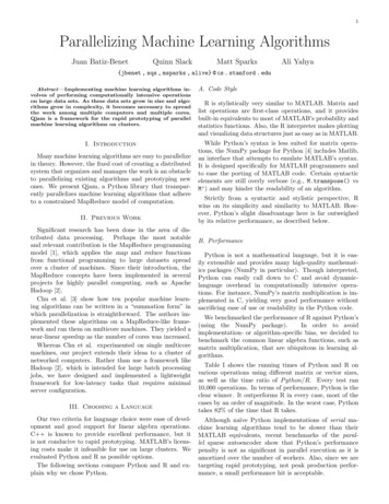
Climate change impact: Recent analyses [48, 28] conclude that the greenhouse gasesemitted from training very large-scale models, such as transformers, can be equivalent to 10years’ worth of individual emissions.1A common alternative is to use smaller-scale datasets, but their value to develop and debug powerfulmethods is limited. For example, image classification datasets such as MNIST [31], SVHN [38] orCIFAR [24] each contain less than 100,000 low-resolution (32 32 pixels) images which enablesshort learning epochs. However, these datasets provide a single task and can prevent insightful modelcomparison since, e.g., modern learning models obtain above 99% accuracy on MNIST.In addition to computational hurdles, fixed datasets limit our ability to explore non-i.i.d. learningparadigms including out-of-distribution generalization, continual learning and, causal inference. I.e.,the algorithms can latch onto spurious correlations, leading to highly detrimental consequenceswhen the evaluation set comes from a different distribution [3]. Similarly, learning disentangledrepresentations requires non i.i.d. data for both training and properly evaluating [34, 20, 46]. Thisraises the need for good synthetic datasets with a wide range of latent features.We introduce Synbols2 , an easy to use dataset generator with a rich composition of latent featuresfor lower-resolution images. Synbols uses Pycairo, a 2D vector graphics library, to render UTF-8symbols with a variety of fonts and patterns. Fig. 1 showcases generated examples from severalattributes (§ 2 provides a complete discussion). To expose the versatility of Synbols, we probe thebehavior of popular algorithms in various sub-fields of our community. Our contributions are: Synbols: a dataset generator with a rich latent feature space that is easy to extend andprovides low resolution images for quick iteration times (§ 2). Experiments probing the behavior of popular learning algorithms in various machinelearning settings including: the robustness of supervised learning and unsupervisedrepresentation-learning approaches w.r.t. changes in latent-data attributes (§ 3.1 and 3.4)and to particular out-of-distribution patterns (§ 3.2), the efficacy of different strategies anduncertainty calibration in active learning (§ 3.3), and the effect of training losses for objectcounting (§ 3.5).Related Work Creating datasets for exploring particular aspects of methods is a common practice.Variants of MNIST are numerous [37, 41], and some such as colored MNIST [3, 2] enable proofs ofconcept, but they are fixed. dSprites [36] and 3D Shapes [21] offer simple variants of 2D and 3Dobjects in 64 64 resolution, but the latent space is still limited. To satisfy the need for a richer latentspace, many works leverage 3D rendering engines to create interesting datasets (e.g, CLEVR [19],Synthia [44], CARLA [10]). This is closer to what we propose with Synbols, but their minimal viableresolution usually significantly exceeds 64 64, which requires large-scale computation.2GeneratorThe objective of the generator is to provide means of playing with a wide variety of concepts in thelatent space while keeping the resolution of the image low. At the same time, we provide a high levelinterface that makes it easy to create new datasets with diverse properties.2.1AttributesFont Diversity (Fig. 1a) To obtain a variety of writing styles, we leverage the large quantity ofartistic work invested in creating the pool of open source fonts available online. When creating anew font, an artist aims to achieve a style that is diversified while maintaining the readability ofthe underlying symbols in a fairly low resolution. This is perfectly suited for our objective. Whilemany fonts are available under commercial license, fonts.google.com provides a repository of opensource fonts.3 This leaves us with more than 1,000 fonts available across a variety of languages. To1This analysis includes hyperparameter search and is based on the average United States energy mix, largerlycomposed of coal. The transition to renewable-energy can reduce these numbers by a factor of 50 [28]. Also,new developments in machine learning can help mitigate climate change [43] at a scale larger than the emissionscoming from training learning ach font family is available under the Open Font License or Apache 2.2
Figure 1: Generated symbols for different fonts, alphabets, resolutions, and appearances.filter out the fonts that are almost identical to each other, we used the confusion matrix from a WideResNet [52] trained to distinguish all the fonts on a large version of the dataset.Different Languages (Fig. 1b) The collection of fonts available at fonts.google.com spans 28languages. After filtering out languages with less than 10 fonts or rendering issues, we are left with14 languages. Interestingly, the Korean alphabet (Hangul) contains 11,172 syllables, each of which isa specific symbol composed of 2 to 5 letters from an alphabet of 35 letters, arranged in a variable 2dimensional structure. This can be used to test the ability of an algorithm to discriminate across alarge amount of classes and to evaluate how it leverages the compositional structure of the symbol.Resolution (Fig. 1c) The number of pixels per image is an important trade-off when building adataset. High resolution provides the opportunity to encode more concepts and provide a widerrange of challenges for learning algorithms. However, it comes with a higher computational costand slower iteration rate. In Fig. 1c-left, we show that we can use a resolution as low as 8 8 andstill obtain readable characters.4 Next, the 16 16 resolution is big enough to render most featuresof Synbols without affecting readability, provided that the range of scaling factors is not too large.Most experiments are conducted in 32 32 pixels, a resolution comparable to most small resolutiondatasets (e.g., MNIST, SVHN, CIFAR). Finally, a resolution of 64 64 is enough to generate usefuldatasets for segmentation, detection and counting.Background and Foreground (Fig. 1d) The texture of the background and foreground is flexibleand can be defined as needed. The default behavior is to use a variety of shades (linear or radial withmultiple colors). To explore the robustness of unsupervised representation learning, we have defineda Camouflage mode, where the color distribution of independent pixels within an image is the samefor background and foreground. This leaves the change of texture as the only hint for detecting thesymbol. It is also possible to use natural images as foreground and background. Finally, we provide amechanism for adding a variety of occlusions or distractions using any UTF-8 symbol.Attributes Each symbol has a variety of attributes that affect the rendering. Most of them areexposed in a Python dict format for later usage such as a variety of supervised prediction tasks, assome hidden ground truth for evaluating the algorithm, or simply a way to split the dataset in a noni.i.d. fashion. The list of attributes includes character, font, language, translation, scale, rotation,bold, and italic. We also provide a segmentation mask for each symbol in the image.2.2InterfaceThe main purpose of the generator is to make it easy to define new datasets. Hence, we providea high-level interface with default distributions for each attribute. Then, specific attributes can beredefined in Python as follows:4For readability, scale and rotation are fixed and solid colors are used for the background and foreground3
s a m p l e r a t t r i b u t e s a m p l e r ( s c a l e 0 . 5 , t r a n s l a t i o n lambda : np . random . u n i f o r m ( 2 , 2 , 2 ) )d a t a s e t d a t a s e t g e n e r a t o r ( sampler , n samples 10000)The first line fixes the scale of every symbol to 50% and redefines the distribution of the x and ytranslation to be uniform between -2 and 2, (instead of -1, 1). The second line constructs a Pythongenerator for sampling 10,000 images. Because of the modified translation, the resulting dataset willhave some symbols partially cropped by the image border. We will see in Sec. 3.3 how this can beuse to study the brittleness of some active learning algorithms.Using this approach, one can easily redefine any attributes independently with a new distribution.When distributions need to be defined jointly, for studying e.g. latent causal structures, we provide aslightly more flexible interface.Datasets are stored in HDF5 or NumPy format and contain images, symbols masks, and all attributes.The default (train, valid, test) partition is also stored to help reproducibility. We also use a combinationof Docker, Git versioning, and random seed fixing to make sure that the same dataset can be recreatedeven if it is not stored.3ExperimentsTo expose the versatility of the dataset generator, we explore the behavior of learning algorithmsacross a variety of machine-learning paradigms. For most experiments, we aim to find a setup underwhich some algorithms fail while others are more resilient. For a concise presentation of results, webreak each subsection into goal, methodology and discussion with a short introduction to providecontext to the experiment. All results are obtained using a (train, valid, test) partition of size ratio(60%, 20%, 20%). Adam [22] is used to train all models, and the learning rate is selected using avalidation set. Average and standard deviation are reported over 3 runs with different random seeds.More details for reproducibility are included in App. ? and the experiments code is available onGitHub5 .3.1Supervised LearningWhile MNIST has been the hallmark of small scale image classification, it offers very minor challenges and it cannot showcase the strength of new learning algorithms. Other datasets such asSVHN offer more diversity but still lack discriminative power. Synbols provides a varying degree ofchallenges exposing the strengths and weaknesses of learning algorithms.Goal: Showcase the various levels of challenges for Synbols datasets. Establish reference points ofcommon baselines for future comparison.Methodology: We generate the Synbols Default dataset by sampling a lower case English characterwith a font uniformly selected from a collection of 1120 fonts. The translation, scale, rotation, bold,and italic are selected to have high variance without affecting the readability of the symbol. Weincrease the difficulty level by applying the Camouflage, and Natural Images feature shown inFig. 1d. The Korean dataset is obtained by sampling uniformly from the first 1000 symbols. Finallywe explore font classification using the Less Variations dataset, which removes the bold and italicfeatures, and reduces the variations of scale and rotation. See App. ? for previews of the datasets.Backbones: We compare 7 models of increasing complexity. Unless specified, all models end withglobal average pooling (GAP) and a linear layer. MLP: A three-layer MLP with hidden size 256and leaky ReLU non-linearities (72k parameters). Conv4 Flat: A four-layer CNN with 64 channelsper layer with flattening instead of GAP, as described by [47] (138k parameters). Conv4 GAP: Avariant of Conv4 with GAP at the output (112k parameters). Resnet-12: A residual network with12 layers [16, 39] (8M parameters). WRN: A wide residual network with 28 layers and a channelmultiplier of 4 [52] (5.8M parameters). Resnet12 and WRN were trained with data augmentationconsisting of random rotations, translation, shear, scaling, and color jitter. More details in App. ?.Discussion: Table 1 shows the experiment results. The MNIST column exposes the lack ofdiscriminative power of this dataset, where an MLP obtains 98.5% accuracy. SVHN offers a marks4
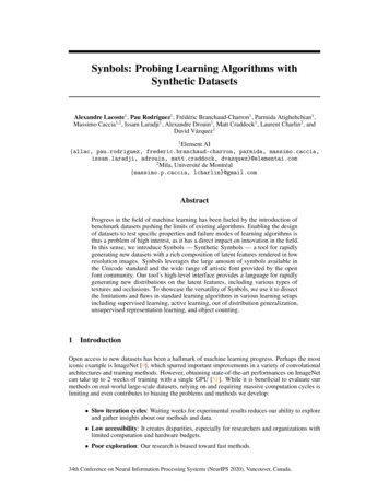
challenge, but the default version of Synbols is even harder. To estimate the aleatoric noise of thedata, we experiment on a larger dataset using 1 million samples. In App. ?, we present an erroranalysis to further understand the dataset. On the more challenging versions of the dataset (i.e.,Camouflage, Natural, Korean, Less Variations) the weaker baselines are often unable to perform.Accuracy on the Korean dataset are surprisingly high, this might be due to the lower diversity of fontfor this language. For font classification, where there is less variation, we see that data augmentationis highly effective. The total training time on datasets of size 100k is about 3 minutes for most models(including ResNet-12) on a Tesla V100 GPU. For WRN the training time goes up to 16 minutes,and about 10 longer for datasets of size 1M.DatasetLabel SetDataset SizeMLPConv-4 FlatConv-4 GAPResNet-12ResNet-12 WRN-28-4WRN-28-4 MNIST10 Digits60k98.5199.3299.0699.7099.7399.6499.74 0.02 0.06 0.07 0.05 0.05 0.06 0.03SVHN10 Digits100k85.0490.7488.3296.3897.1996.0797.30 0.21 0.27 0.21 0.03 0.04 0.07 0.05Synbols Default48 Symbols48 Symbols100k1MCamouflage48 Symbols100kNatural48 Symbols100kKorean1000 Symbols100kLess Variations1120 Fonts100k14.8368.5170.1495.4397.1693.5797.414.08 0.0832.35 1.5129.60 0.5590.14 0.0594.09 0.0786.34 0.1695.55 0.255.02 0.0819.43 1.0125.60 1.0581.21 0.4685.80 0.1573.26 0.5388.30 0.230.12 0.021.62 0.1333.58 4.6597.08 0.1398.54 0.0795.79 0.5199.14 0.090.11 0.030.21 0.043.16 0.3839.41 0.3057.42 0.5023.10 0.9068.42 1.11 0.40 0.66 0.41 0.12 0.05 0.29 0.0463.0589.4590.8798.8599.4498.8899.57 0.80 0.19 0.11 0.02 0.00 0.04 0.01Table 1: Supervised learning: Accuracy of various models on supervised classification tasks. Resultswithin 2 standard deviations of the highest accuracy are in bold.3.2Out of Distribution GeneralizationThe supervised learning paradigm usually assumes that the training and testing sets are sampledindependently and from the same distribution (i.i.d.). In practice, an algorithm may be deployed in anenvironment very different from the training set and have no guarantee to behave well. To improvethis, our community developed various types of inductive biases [53, 12], including architectures withbuilt-in invariances [30], data augmentation [30, 25, 8], and more recently, robustness to spuriouscorrelations [3, 1, 26]. However, the evaluation of such properties on out-of-distribution datasets isvery sporadic. Here we propose to leverage Synbols to peek at some of those properties.Goal: Evaluate the inductive bias of common learning algorithms by changing the latent factordistributions between the training, validation, and tests sets.Figure 2: Example of the different types of split using scale and rotationMethodology: We use the Synbols Default dataset (Sec. 3.1) and we partition the train, validation,and test sets using different latent factors. Stratified Partitions uses the first and last 20 percentiles ofa continuous latent factor as the validation and test set respectively, leaving the remaining samplesfor training (Fig. 2). For discrete attributes, we randomly partition the different values. Solvingsuch a challenge is only possible if there is a built-in invariance in the architecture. We also proposeCompositional Partitions to evaluate the ability of an algorithm to compose different concepts. Thisis done by combining two stratified partitions such that there are large holes in the joint distributionwhile making sure that the marginals keep a comparable distribution (Fig. 2-right).Discussion: Results from Table 2 show several drops in performance when changing the distributionof some latent factors compared to the i.i.d. reference point highlighted in blue. Most algorithms arebarely affected in the Stratified Font column. This means that character recognition is robust to fonts5
DatasetPartitionMLPConv-4 FlatConv-4 GAPResnet-12Resnet-12 WRN-28-4WRN-28-4 i.i.d.14.8368.5170.1495.4397.1693.5797.41 .40 .66 .41 .12 .05 .29 41 .37 .68 .18 .09 .06 .11 .08Synbols 62.8594.1096.3492.1896.80 .35 .17 .37 .13 .07 .16 .1411.41 .055.54 .3148.25 .3882.37 .0391.96 .3079.53 .0991.81 ss VariationsStratifiedChar7.91 .2153.87 .8954.88 .5790.56 .2094.43 .2687.68 .4695.16 .067.96 .0644.78 .7265.46 .3794.62 .1996.84 .0792.99 .0797.33 .16.08 .01.24 .012.97 .3225.59 .2233.95 .6116.85 .2335.41 2.39Table 2: Out of Distribution: Results reporting accuracy on various train, valid, test partitions.Results in blue are the reference point for the Synbols Default dataset, results in red have a drop ofmore than 5% absolute accuracy compared to reference point, and bold results have a drop of lessthan 0.5% absolute accuracy compared to reference point. Refer to Table 1 for the reference point offont classification on the Less Variations dataset.that are out of distribution.6 On the other hand, all architectures are very sensitive to the StratifiedRotation partition, suffering from a systematic drop of at least 5% absolute accuracy compared tothe i.i.d. evaluation. While data augmentation helps it still suffers from an important drop of accuracy.Scale is also a factor that affects the performance, but interestingly, some architectures are muchmore resilient than others.7 Next, the Compositional Rot-Scale partition shows less performancedrop than its stratified counterparts. This hints that neural networks are capable of some form ofcompositional learning. Moving on to the Stratified x-Translation partition, we see that manyalgorithms not affected by this intervention and retains its original performance. This is expectedsince convolution with global average pooling is invariant to translation. However, the MLP andConv-4 Flat do not share this property and they are significantly affected. Finally, we observe animportant drop of performance on font prediction when it is evaluated on characters that were notseen during training. This hints that many font classification results in Table 1 are memorizing pairsof symbols and font.3.3Active LearningInstead of using a large supervised dataset, active learning algorithms aim to request labels for a smallsubset of unlabeled data. This is done using a query function seeking the most informative samples.A common query function is the predictive entropy (P-Entropy) [45]. However, a more principledmethod uses the mutual information between the model uncertainty and the prediction uncertainty ofa given sample. This can be efficiently approximated using BALD [18]. However, in practice, it iscommon to observe comparable predictive performances between BALD and P-Entropy [5, 13]. Wehypothesize that this may come from the lack of aleatoric uncertainty in common datasets. We thusexplore a variety of noise sources, ranging from pixel noise to ablative noise in the latent space. Wealso explore the importance of uncertainty calibration using Kull et al. [27]. This is done by learninga Dirichlet distribution as an extra layer after the logits, while keeping the rest of the network fixed.To look at the optimistic scenario, we learn it using the full validation set with all the labels (after thenetwork has converged using its labeled set).Goal: Showcase the brittleness of P-Entropy on some types of noise. Search for cases where BALDmay fail and see where calibrated uncertainty can help.Methodology: We compare BALD and P-Entropy to random sampling. These methods are evaluated on different variations of Synbols Default. The Label Noise dataset introduces uniform noise inlabels with probability 0.1. The Pixel Noise dataset adds N (0, 0.3) to each pixel in 10% of theimages and clips back the pixel value to the range (0, 1). The 10% missing dataset omits the symbolwith probability 0.1. In the Cropped dataset, translations are sampled uniformly between -2 and 2,yielding many symbols that are partly cropped. Finally, the 20% Occluded dataset draws a largeshape, occluding part of the symbol with probability 0.2. For concise results, we report the NegativeLog Likelihood after labeling 10% of the unlabeled set. Performance at 5% and 20% labeling sizecan be found in Sec. ?, along with implementation details and previews of all datasets.67This is not too surprising since there is a large amount of fonts and many share similarities.The test partition uses larger scale which tend to be easier to classify, leading to higher accuracy.6
CIFAR10BALDP-EntropyRandomBALD CalibratedEntropy Calibrated0.59 0.030.59 0.010.66 0.040.58 0.010.57 0.02No Noise0.850.850.980.890.86 0.09 0.06 0.05 0.08 0.07Label NoisePixel Noise2.052.032.122.001.990.911.451.000.931.42 0.06 0.04 0.11 0.04 0.06 0.02 0.06 0.04 0.03 0.0410% Missing1.242.021.321.192.06 0.04 0.05 0.07 0.08 0.05Out of the Box1.962.482.042.002.51 0.03 0.04 0.04 0.08 0.0420% Occluded1.391.721.511.381.66 0.05 0.09 0.04 0.05 0.05Table 3: Active Learning results reporting Negative Log Likelihood on test set after labeling 10% ofthe unlabeled training set. Results worse than random sampling are shown in red and results within 1standard deviation of the best result are shown in bold.Discussion: In Table 3, we recover the result where P-Entropy is comparable to BALD usingCIFAR 10 and the No Noise dataset. Interestingly, the results highlighted in red show that P-Entropywill perform systematically worse than random when some images have unreadable symbols whileBALD keeps its competitive advantage against Random. When training on 10% Missing, we foundthat P-Entropy selected 68% of it’s queries from the set of images with omitted symbols vs 4% forBALD. We also found that label noise and pixel noise are not appropriate to highlight this failuremode. Finally, calibrating the uncertainty on a validation set did not significantly improve our results.3.4Unsupervised Representation LearningUnsupervised representation learning leverages unlabeled images to find a semantically meaningfulrepresentation that can be used on a downstream task. For example, a Variational Auto-Encoder(VAE) [23] tries to find the most compressed representation sufficient to reconstruct the originalimage. In Kingma and Welling [23], the decoder is a deterministic function of the latent factors withindependent additive noise on each pixel. This inductive bias is convenient for MNIST where there isa very small amount of latent factors controlling the image. However, we will see that simply addingtexture can be highly detrimental on the usefulness of the latent representation. The HierarchicalVAE (HVAE) [54] is more flexible, encoding local patterns in the lower level representation andglobal patterns in the highest levels. Instead of reconstructing the original image, Deep InfoMax [17]optimizes the mutual information between the representation and the original image. As an additionalinductive bias, the global representation is optimized to be predictive of each location of the image.Goal: Evaluate the robustness of representation learning algorithms to change of background.Methodology: We generate 3 variants of the dataset where only the foreground and backgroundchange. To provide a larger foreground surface, we keep the Bold property always active and varythe scale slightly around 70%. The other properties follow the Synbols Default dataset. The SolidPattern dataset uses a black and white contrast. The Shades dataset keeps the smooth gradient fromDefault Synbols. The Camouflage dataset contains many lines of random color with the orientationdepending on whether it is in the foreground or the background. Samples from the dataset can be seenin Sec. ?. All algorithms are then trained on 100k samples from each dataset using a 64-dimensionalrepresentation. Finally, to evaluate the quality of the representation on downstream tasks, we fix theencoder and use the training set for learning an MLP to perform classification of the 26 characters orthe 888 fonts. For comparison purposes, we use the same backbone as Deep InfoMax for our VAEimplementation and we also explore using ResNet-12 for a higher capacity VAE.Deep InfoMaxVAEHVAE (2 level)VAE ResNetHVAE (2 level) ResNetCharacter AccuracySolid PatternShadesCamouflageSolid Pattern83.8763.4866.7274.1672.1916.44 0.672.68 0.152.71 0.534.97 0.083.33 0.06 0.80 0.97 9.36 0.37 0.116.52 0.6022.43 2.6528.86 1.1737.40 0.4658.36 3.454.853.853.913.333.52 2.01 0.33 0.19 0.02 0.16Font AccuracyShadesCamouflage0.310.360.390.550.73 0.04 0.07 0.10 0.04 0.160.280.180.170.170.16 0.10 0.01 0.01 0.03 0.02Table 4: Unsupervised Representation Learning: Results reporting classification accuracy on 2downstream tasks. Highest performance is in bold and red exposes unexpected results.Discussion: While most algorithms perform relatively well on the Solid Pattern dataset, we canobserve a significant drop in performance by simply applying shades to the foreground and background. When using the Camouflage dataset, all algorithms are only marginally better than randompredictions. Given the difficulty of the task, this result could be expected, but recall that in Table 1,adding camouflage hardly affected the results of supervised learning algorithms. Deep InfoMax7
is often the highest performer, even against HVAE with a higher capacity backbone. However theperformances on Camouflage are still very low with high variance indicating instabilities. Surprisingly, Deep InfoMax largely underperforms on the Shades dataset. This is likely due to the globalstructure of the gradient pattern, which competes with the symbol information in the limited sizerepresentation. This unexpected result offers the opportunity to further investigate the behavior ofDeep InfoMax and potentially discover a higher performing variant.3.5Object CountingObject counting is the task of counting the number of objects of interest in an image. The task mightalso include localization where the goal is to identify the locations of the objects in the image. Thistask has important real-life applications such as ecological surveys [4] and cell counting [7]. Thedatasets used for this task [14, 4] are often labeled with point-level annotations where a single pixelis labeled for each object. There exists two main approaches for object counting: detection-based anddensity-based methods. Density-based methods [32, 33] transform the point-level annotations into adensity map using a Gaussian kernel. Then they are trained using a least-squares objective to predictthe density map. Detection-based methods first detect the object locations in the images and thencount the number of detected instances. LCFCN [29] uses a fully convolutional neural network and adetection-based loss function that encourages the model to output a single blob per object.Goal: We compare between an FCN8 [35] that uses the LCFCN loss and one that uses the densityloss function. The comparison is based on their sensitivity to scale variations, object overlapping, andthe density of the objects in the images.Methodology: We generate 5 datasets consisting of 128 128 images with a varying number offloating English letters on a shaded background. With probability 0.7, a letter is generated as ‘a’,otherwise, a letter is uniformly sampled from the remaining English letters. We use mean absoluteerror (MAE) and grid average mean absolute error (GAME) [15] to meas
Progress in the field of machine learning has been fueled by the introduction of benchmark datasets pushing the limits of existing algorithms. Enabling the design of datasets to test specific properties and failure modes of learning algorithms is thus a problem of high interest, as it has a direct impact on innovation in the field.