Transcription
Portfolio Optimization with Transaction CostsA Major Qualifying Project ReportSubmitted to the Faculty ofWORCESTER POLYTECHNIC INSTITUTEIn partial fulfillment of the requirements for theDegree of Bachelor of SciencebyJessica M. ClarkSean E. MulreadyApproved:Professor Arthur Heinricher, AdvisorAPRIL 26, 2007
Contents1 Introduction12 Background2.1 Basic Portfolio Analysis . . . . .2.2 Portfolio Optimization . . . . . .2.2.1 Risk versus Return . . . .2.2.2 Efficient Portfolios . . . .2.2.3 Fully Invested Constraint.3355673 Constraints3.1 Booksize . . . . . . . . . . . . . . . . . . . . . . . . . . . . . . . .3.2 Turnover and Transaction Costs . . . . . . . . . . . . . . . . . .99104 Implementation of Portfolio Optimization4.1 Constraint Linearization . . . . . . . . . . .4.2 Proof of Validity of Linearization . . . . . .4.3 Standard Constraint Formulation . . . . . .4.4 Description of Algorithm . . . . . . . . . . .12121315175 Results5.1 Data Management . . . . . . . . . . . . . .5.1.1 Source of Data . . . . . . . . . . . .5.1.2 Definition of Time Periods . . . . . .5.1.3 Verifying Validity of Optimization .5.2 Evolution of Portfolios . . . . . . . . . . . .5.3 Portfolio Value Calculations . . . . . . . . .5.4 Comparing Value and Utility Plots . . . . .5.4.1 Efficient vs. Equally Weighted Plots5.4.2 Booksize Plots . . . . . . . . . . . .5.4.3 Turnover Plots . . . . . . . . . . . .1919191920202122222224.6 Explorations296.1 Turnover Budgeting . . . . . . . . . . . . . . . . . . . . . . . . . 296.2 Threshold Trading . . . . . . . . . . . . . . . . . . . . . . . . . . 30i
7 Conclusion348 Appendices368.1 Appendix A: MatLab Code . . . . . . . . . . . . . . . . . . . . . 368.2 Appendix B: PowerPoint Presentation . . . . . . . . . . . . . . . 47ii
AbstractInvestors often update their portfolios at regular time intervals by trading stocks, but there are costs associated with these trades. This project seeksto limit these transaction costs by controlling the portfolio turnover (absolutechange as a fraction of book size) between time periods. The result is a multiperiod optimization problem with quadratic objective function and non-smoothconstraints. The resulting portfolios outperformed benchmark portfolios in bothexpected utility and actual portfolio value.iii
Chapter 1IntroductionInvestors often update their stock portfolios at regular time intervals, buying and selling stocks to maximize expected return while also minimizing risk.One standard approach is minimize a utility function incorporating both riskand return, typically with a parameter to measure risk tolerance and additionalconstraints.[3] In traditional portfolio optimization, the sum of the fraction invested in each stock is constrained. If short-selling is allowed, then it is usefulto instead constrain the booksize, the sum of the absolute values of the weights.This mathematical framework allows investors to select an optimal (or at leastefficient) portfolio at any given time.In practice, portfolios are held for long time periods and are adjusted, orre-optimized at specific intervals. While Markowitz [3] showed how to find thebest portfolio at a given time, the basic formulation does not include the costsassociated with changing the weights in the portfolio. Each transaction has anassociated cost and these costs must be included in the decision process.It is difficult to model these costs, because they can depend on many factors1
including the size of the trade and the type of asset being traded. One way tolimit transaction costs is by introducing a constraint on turnover, the sum ofthe absolute differences in weights between adjacent time periods. The goalsof this project were to implement a portfolio optimization algorithm with bothbooksize and turnover constraints and to explore the effects of the turnoverconstraint on portfolio value and utility in a multi-period setting.The objective function of the portfolio optimization problem is quadratic;however, the constraints on booksize and turnover are nonlinear and non-smooth.Since standard quadratic programming packages require linear constraints, theconstraints were linearized by splitting the variables.The optimization algorithm was tested on a set of four stocks over eleventime periods. Both the expected utility and actual performance of the resulting portfolios were compared to those of unconstrained and equally weightedportfolios. The optimal portfolios typically outperformed the equally weightedportfolios. Comparisons were also made of the performance of portfolios withdifferent allowances of booksize and turnover.With turnover constraints in place, the ideas of turnover budgeting andthreshold trading were developed and tested. Turnover budgeting allows dynamic allocation of turnover across multiple time periods. Threshold tradinglimits trading subject to criteria on the expected change in utility. These andother extensions of the turnover constraint can be used to model and limittransaction costs in more realistic ways.2
Chapter 2Background2.1Basic Portfolio AnalysisThere are two main problems in portfolio analysis: estimation and optimization. The estimation problem is basically the problem of forecasting investmentreturn. In a sense this, is a statistical or econometric problem and it is the mostdifficult of the two problems. If a manager has very good forecasts for stockbehavior, investment decisions are very easy.The focus of this project is almost entirely on the optimization problem.Given a set of data and some basic statistics computed from that data, whatis the optimal portfolio choice? How can the investor balance the goal of highreturn against the challenge of large risks? This view, the idea that investorsbalance return and risk, was the insight of Harry Markowitz and his view is thefoundation for Mean–Variance analysis in portfolio management.This project considers the situation where an investor is choosing amonga set of n stocks in which to invest. This set of stocks can be represented as ann 1 vector. Let this vector be denoted as x. Then, xi is the number of shares3
invested in asset i.Notice that the entries in x can be positive, 0, or negative. If xi 0,then the investor owns a positive number of shares in asset i. If xi 0, thenthe investor has a short position in asset i. This means that the investor hasborrowed shares of stock from someone else, sold them, and kept the proceedsfrom the sale. At some point in the future, the investor will have to buy theshares of stock back and give them to the original owner. This is called closingthe short position. Clearly, short selling is done with the hope that the stockwill drop in price. If xi 0, the investor owns no shares of stock i.To further illustrate the idea of short selling, consider investor A andinvestor B. Assume that Microsoft stock is worth 30 per share today. InvestorA thinks that Microsoft will go down in the next week, so he borrows 10 sharesof Microsoft stock from investor B and sells them immediately, collecting 300.If Microsoft stock drops to 20 per share next week, investor A can buy the 10shares back for 200 and close his short position with B by giving the sharesback. Investor A would make a profit of 100 from this transaction. However,if Micosoft stock goes up, A will lose money. For instance, if Microsoft is worth 60 next week, it will cost A 600 to buy the stocks back and close the position,earning him a net loss of 300. For this reason, short selling is riskier than onlybuying stocks because the possible amount of loss is unbounded. Stock pricescannot drop below 0 per share, but they can go up almost indefinitely.4
2.22.2.1Portfolio OptimizationRisk versus ReturnInvestors want to choose their portfolio to minimize risk while simultaneouslyobtaining the maximum amount of return. These two objectives can sometimesoppose each other. For instance, consider the portfolio where all of the investor’smoney is invested in the stock that he thinks will perform the best. Althoughthis portfolio has a high amount of expected return, it also is very risky, becauseif that one stock drops, the investor does not have any other assets that couldmake up for it. On the other hand, if an investor invests equally in all possiblestocks, he is not taking advantage of any stocks that will probably performbetter than others.Economists have long studied the ways that investors attempt to balancerisk versus return, but it was Harry Markowitz [3] who first defined risk asvariance in portfolio return.Risk xT Ω x Xxi σij xj(2.1)i,jReturn µ T x Xµi xi(2.2)iwhere Ω is the (n n) covariance matrix for the assets and µ is the ((n 1)vector of returns. These are estimated from historical data for stock prices.5
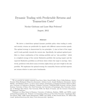
2.2.2Efficient PortfoliosThere is not a single portfolio which is “optimal” for all investors. Differentinvestors have different levels of risk tolerance and are willing to carry morerisk for the chance of obtaining more return. It is, however, possible to identifyportfolios which an investor should consider.An efficient portfolio has the lowest risk for a given return, as well as thehighest return for that amount of risk [3].Efficient portfolios are found by solving the optimization problemMinimize xT Ω x 1 Tµ xλ(2.3)where λ is a parameter representing the investor’s risk tolerance. If λ is large,then1λwill be close to zero, meaning that the investor does not have much risktolerance (most of the emphasis in the optimization problem is placed on risk).Conversely, if λ is small, then1λwill be large, placing more emphasis on return.The efficient frontier is the curve made up of all efficient portfolios. Itis calculated by running the above optimization over many values of λ, andvisualized by plotting all of the efficient frontiers in risk-return space, as infigure 2.1 [3].The efficient frontier can be interpreted as the collection of all portfoliosthat have the highest risk for a given amount of return, as well as the highestreturn for that amount of risk. In figure 2.1, notice that portfolio a is not on theefficient frontier because one can achieve a higher amount of return for the sameamount of risk with portfolio b, and a lower amount of risk for the same amount6
Figure 2.1: Sample Efficient Frontierof return with portfolio c. Also notice that in order to get a large amount ofreturn, one must be willing to take on a lot of risk, and to get a very smallamount of risk, one must be able to accept low expected return.2.2.3Fully Invested ConstraintA constraint that is commonly placed on the classical portfolio optimizationproblem is called the Fully Invested constraint, which requires that the amountof money invested in the portfolio is equal to some number F. This can be viewedas a requirement that the investor buys only the number of stocks he wants to,while not exceeding that number of stocks. With the fully invested constraintadded, the optimization problem becomes:Minimize xT Ω x 71 Tµ xλ(2.4)
nXs.t.xi F(2.5)i 1The fully invested constraint is typically used for problems where short selling is not allowed. As is shown in the next section, the fully invested constraintis not very meaningful when applied to portfolios where short selling is allowed.8
Chapter 3Constraints3.1BooksizeIn classic portfolio optimization, there typically exists a fully invested constraint, which sets the sum of the porfolio weights equal to a constant. As ourmodel allows for short-selling, xi 0, this constraint is not very meaningful.Instead, this approach limits the sum of the absolute value of portfolio weights,or the booksize.Booksize nX xi M(3.1)i 1Here’s a simple two-stock example to illustrate the importance of booksizewhen short-selling is allowed:At time 0, there are two stocks, each priced at 10 per share. Say someonebuys ten shares of Stock 1 and sells-short ten shares of Stock 2. To purchase theten shares of Stock 1, the person withdrew 100 from a bank account. However,when selling-short in Stock 2, he received that 100 back. Therefore, his net 10change in wealth is 0. The position vector becomes x . Notice the 109
sum of the weights equals 0. Also the booksize is 20.At time 1, things go bad for the investor. Stock 1 drops in price to 5per share while Stock 2 increases to 15 per share. The investor decides to sellhis shares in Stock 1 and close his position in Stock 2. By selling Stock 1, theinvestor gains 50. However, to close his position in Stock 2, the investor mustwithdraw 150. The investor now has a net change in wealth of - 100. Thisloss could not have been predicted by examining only the net weight in shares,which equalled 0. This shows the importance of booksize with regards to theamount of money at risk for loss.3.2Turnover and Transaction CostsThere are three types of transaction costs associated with every trade: commission, the bid/ask spread, and market impact. Commission is the amount abroker charges for performing a trade, which can be a set price or depend onthe size of the trade. The bid/ask spread is the difference in price at which onecan buy a share of stock and then immediately sell it. The market impact is thecost associated with trading several shares of a stock, i.e. changing the priceof the stock. There is also a fourth type of transaction cost called opportunitycost which measures the amount lost for not trading a particular stock. [2]An investor may want to limit the amount that the portfolio changesover time, because of the transaction costs associated with changing the portfolio(buying and selling assets). The turnover constraint is introduced to accomplishthis.10
The turnover is the sum of the absolute values of the difference between eachposition at time t and time t 1.Turnover(t) nX xi (t) xi (t 1) (3.2)i 1where xi (t) refers to the position in asset i at time t and xi (t 1) refers tothe position in asset i at time t 1.The turnover is constrained by requiring that it is less than or equal to someconstant, typically between 0 and 1, multiplied by the booksize of the portfolioat time t 1.nX xi (t) xi (t 1) Li 1nX xi (t 1) (3.3)i 1The optimization problem is then:Minimizes.t.nP T x xT Ω x λ1 µ xi M(3.4)i 1nPi 1 xi xoldi L11nPi 1 xoldi
Chapter 4Implementation of PortfolioOptimization4.1Constraint LinearizationNotice that the optimization has a quadratic objective function, so it wouldbe efficient and effective to use a standard quadratic programming tool (such asMatLab’s quadprog); however, standard quadratic programming tools requirelinear constraints. The booksize and turnover constraints are nonlinear becausethe sums of absolute values are being calculated. The constraints were there fore linearized by splitting each xi into two new variables, b i and bi for thebooksize constraint, and yi and yi for the turnover constraint. Introducingsplit variables transforms the problem into the following standard quadraticprogramming problem:Minimize xT Ω x 121 Tµ xλ
s.t. xi b i bib i 0nXb i 0 b i bi Mi 1xi yi yi yi 0nXyi 0nXyi yi L xoldi i 1i 1 An interpretation of the booksize split variables (b i and bi ) is thatb i b i xi c,d,c, xi d,if xi 0if xi 0if xi 0if xi 0where c and d are constants. This interpretation says that the split variablesare the positive and negative components of each xi , respectively, shifted bya constant. The interpretation is the same for the turnover constraint’s splitvariables.4.2Proof of Validity of Linearization Let x (x1 , . . . , xn ), b (b 1 , . . . , bn ), b (b1 , . . . , bn ).Define two sets. Let ( x, b , b )s.t. x b i bi , (for each i) i bi 0,A : b i 0, n P bi b i Mi 113 (4.1)
LetB : { x s.t.nX xi M }(4.2)i 1We want to show that minimizing utility for A is the same as minimizingutility for B. To do this, we show that x B, (b , b ) such that ( x, b , b ) A, and that ( x, b , b ) A, x B.Let x B be given. ThennP xi M . We need to show that we can findi 1 b , b such that ( x, b , b ) A.For each i, letb ib i : : xi ,0,if xi 0if xi 00, xi ,if xi 0if xi 0 Then, xi b i bi , bi 0, bi 0, and bi bi xi M and sonPi 1 b x B, then there exists b , b suchi bi M and this implies that if that ( x, b , b ) A. Next, let A ( x, b , b ) A be given. Then xi b i bi , bi 0, bi 0,nPi 1 b i bi M . Notice:nXi 1xi nX b i bi i 1nX b i bi Mi 1 Because for each i, b i 0, bi 0. There are two cases: xi 0, and xi 0.14
Case (i): xi 0 xi xi b i biCase (ii): xi 0 x x b i bi bi biwhich implies thatnXxi i 1nX b i bi M.i 1Henceif ( x, b , b ) A, x B.Therefore, the set of feasible x is the same for each set, so minimizing theobjective function over one set will yield the same result as minimizing over theother.4.3Standard Constraint FormulationMatLab’s QuadProg package minimizes the function xT H x f T x, subject to the constraints A x b, and Aeq x beq, where H, A, and Aeq are k k square matrices, and f , b and beq are k 1 vectors (k is the number of decisionvariables). In this project, QuadProg is run on the optimization problem:Minimize xT Ω x 1 Tµ xλ s.t. xi b i bib i 0nXb i 0 b i bi Mi 115
xi yi yi yi 0nXyi 0nXyi yi L xoldi i 1i 1First, the matrices H, A, and Aeq need to be augmented to allow for thesplit constraint variables. These variables will be in the objective function, butthey should not have any impact on the objective function value. Therefore, if nis the number of stocks in the portfolio, then augment H with 4n zeros in eachrow and column, so that it will be a square matrix with dimensions 5n 5n.Similarly, augment f with 4n zeros, so that it is a vector with dimensions 5n 1.The inequality and equality constraints need to be translated into matrixand vector form. The constraints are rearranged so that all decision variables areon the left side, and all inequalities are “less than or equal to”. The (rearranged) list of inequality constraints is: b i 0, bi 0,0, yi ,nPi 1yi yi LnPi 1 xoldi .nPi 1 b i bi M, yi The list of equality constraints is: xi b i bi 0, xi yi yi 0. Now, the matrices A and Aeq, and the vectors b and beq can be defined. Let 0 denote an n n matrix of zeros, I denote ann n identity matrix, 0 denote an n 1 matrix of zeros, and 1 denote an n 1matrix of ones. A 0 I000000 T01T 0T 0T0 I00 1T 0T00 I0 0T 1T000 I 0T 1T ,b 0 0 0 0MnPL xoldi i 116
Aeq I II0 I00I0 I , beq 0 xOld Each column of A and Aeq corresponds to a vector of decision variables. Thefirst corresponds to x, the second to b , the third to b , the fourth to y ,and the fifth to y . Also, every row corresponds to a constraint. With theconstraints in a standard linear form, QuadProg can be used in the followingway to perform portfolio optimization.4.4Description of AlgorithmInputs:λ risk toleranceL turnover constraint parameterM booksize constraintChoose which constraints to use (none, booksize only, turnover only, booksize and turnover)Choose what to plot (portfolio weights, portfolio utility, portfolio value) Obtain the data (get risk matrices and return vectors for each time step). numStocks the number of stocks in the portfolio numT imeP eriods the number of time periods for which to optimize xOld equally weighted portfolio of numStocks stocks17
for i 1 to numTimePeriods– select appropriate µ and ω– run quadprog with linearized constraints to find x– xOld x Plot portfolio weights, utility, and value as requested18
Chapter 5Results5.15.1.1Data ManagementSource of DataThe data used in this project was downloaded from Yahoo Finance. Itconsists of daily closing prices of stocks over an 80-day period. Four stockswere selected that are known to have low volatility: Gap, Lucent Technologies,Verizon Communications, and Disney. Also four stocks that are known for theirhigh volatility were selected: DayStar Technologies, Salesforce.com, BriteSmile,and iMergent. For each sets of stocks, the daily returns were used to computethe µ (average return) and Ω (risk) matrices.5.1.2Definition of Time PeriodsThe turnover constraint is implemented over several time periods. Therefore,to test the constraint several time periods worth of data were generated. Elevenµ and eleven Ω matrices were calculated using 30 days worth of data for eachperiod shifted five days. The optimization problem was solved across all of thetime periods.19
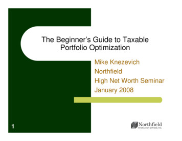
5.1.3Verifying Validity of OptimizationTo further verify the linearization of the constraints, the unconstrained problem was solved with a set of four stocks and compared to a loosely constrainedproblem on the same set of stocks. Constraints were chosen that would be satisfied by the solution to the unconstrained problem, i.e., allowing large booksizesand amounts of turnover between time periods. On each set of stocks, the solution to the unconstrained problem was identical to the solution of the looselyconstrained problem. This provided further verification that the linearizationof the constraints was valid.5.2Evolution of PortfoliosFigure 5.1 shows the evolution a portfolio over 11 time periods with constraints on booksize and turnover. The algorithm defaulted to an equallyweighted portfolio in the first time period. In this example, the booksize is10.There are several important features about the dynamics of the portfolioshown by Figure 5.1. The constraint on booksize limits portfolio booksize lessthan or equal to a particular value. Between the first two time period thebooksize actually decreases in value. By the final time step our booksize hasdecreased in value from 10 to 7. Between each time step, there is a certainamount turnover conducted by the algorithm. As the portfolio evolves throughtime steps, the distribution in weights of the portfolio becomes increasinglydifferent from the original portfolio. Finally, the weight of dark blue stock in20
Portfolio Weights43.532.5Weight21.510.50 0.5 1Time PeriodFigure 5.1: Evolution of Portfolio Weightsthe middle time periods become negative values, reiterating the allowance ofshort-selling.5.3Portfolio Value CalculationsPortfolio value is defined as the amount of money an investor would have ifhe sold all his stocks and closed all his short positions plus all of his earnings.Let wi (t) represent the price of stock i at time t, wi xi be the current wealth ofstock i, M M A equal the amount of money in bank, M M Ai (t) symbolize the21
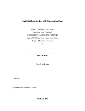
change in balance from time t 1 to time t, and Value(t) be the portfolio value.At time t, the change in balance caused by stock i is going to equal thechange in weights from time t 1 to time t multiplied by the price of stock iat time t. More generally, the overall change will equal the dot product of thevector of prices and the vector of change in weights.hi M M A(t) w T (t) x(t) x(t 1)(5.1)The current balance M M A will equal the sum of all changes in balance. Portfolio value will equal the current balance plus the present wealth of the portfolio.V alue(t) w T (t) x(t) M M A n X wi (t)xi (t) M M A(5.2)i 15.45.4.1Comparing Value and Utility PlotsEfficient vs. Equally Weighted PlotsTo evaluate the performance of our portfolio, it was compared to a portfolio that was equally weighted at each time step. In Figure 5.2 the efficientportfolio either matched or exceeded the equally-weighted portfolio in actualperformance. As shown in Figure 5.3, the efficient portfolio easily outperformedthe equally-weighted portfolio in expected utility.The next set of graphs are explorations of the effects of different allowancesof booksize and turnover.5.4.2Booksize PlotsFirst, the algorithm was run for different allowances of booksize. Figure 5.4illustrates the principle that generally relaxing the booksize allows for greater22
Portfolio Value Efficient vs. Equally Weighted230Efficient PortfolioEqually Weighted PortfolioConstraints:M 10 (Booksize)L 1 (Turnover)220210Portfolio Value2001901801701601501401234567891011Time PeriodFigure 5.2: Portfolio Value: Efficient vs. Equally Weightedreturn (and as a result portfolio value).Figure 5.5 shows the expected utility of the same portfolios. The results arecounterintuitive. A portfolio with a loosely constrained booksize has a greaterset of feasible portfolios than a portfolio with a tightly constrained booksize.Actually, the smaller set is a subset of the larger set. However, since there is aconstraint on turnover, these sets no longer necessarily intersect. As a result, itis possible to obtain a better utility with a more tightly constrained booksize.23
Portfolio Utility Efficient vs. Equally Weighted0.06Efficient PortfolioEqually Weighted PortfolioConstraints:M 10 (Booksize)L 1 (Turnover)0.04Portfolio Utility0.020 0.02 0.04 0.06 0.08024681012Time PeriodFigure 5.3: Portfolio Utility: Efficient vs. Equally Weighted5.4.3Turnover PlotsNext the algorithm was run for different allowances of turnover (Figure 5.6).Judging by the latter time periods, it appears that allowing larger amountsin turnover is a great idea. These results are deceiving as the calculation ofportfolio value does not consider transaction costs.Figure 5.7 shows the expected utility of the previous portfolios. This graphmay also seem counterintuitive, similar to the utility plot of different booksizes.24
Portfolio Value with Different Booksizes260M 30240M 10M 5M 1Portfolio Value2202001801601401234567891011Time PeriodFigure 5.4: Portfolio Value for Different BooksizesIt is important to note that similar utility does not imply similar portfolio. Inthe first time step, it is possible for a loosely constrained portfolio to makean enormous change in its distribution of weights, while a tightly constrainedportfolio will not. As a result, in the second time step the tightly constrainedportfolio might be closer to achieve a portfolio with good utility. In fact, theloosely constrained portfolio may only be able to achieve a portfolio with poorutility. As a result, the tightly constrained portfolio may outperform the looselyconstrained one. Even without considering transaction costs, allowing large25
Portfolio Utility for Different Booksizes0 0.01 0.02Utility 0.03 0.04M 30M 10 0.05M 5M 1 0.06 0.07024681012Time PeriodFigure 5.5: Portfolio Utility for Different Booksizesamounts of turnover is a bad idea since your portfolio may not be able toconsistently achieve good utility.26
Portfolio Value for Different Allowances of Turnover240230L 1L 0.50220L 0.25L 0.10Portfolio Value2102001901801701601501401234567891011Time PeriodFigure 5.6: Portfolio Value for Different Allowances of Turnover27
Portfolio Utility for Different Allowances of Turnover0.01L 1L 0.50L 0.25L 0.100 0.01Utility 0.02 0.03 0.04 0.05 0.06 0.07024681012Time PeriodFigure 5.7: Portfolio Utility for Different Allowances of Turnover28
Chapter 6ExplorationsOnce the turnover and booksize constraints were implemented, it was possible toextend the idea of constraining turnover to limit transaction costs in two moreways. The first, called turnover budgeting, involves dynamically implementingturnover at different time steps. The second, called threshold trading, involvesonly trading if the expected change in utility is large enough.6.1Turnover BudgetingWith turnover budgeting, the basic idea is that a different amount of turnoveris allowed at each time step. This translates to the parameter L in the turnoverconstraint being different at different times. One way to demonstrate this ideais to consider a set of eleven time periods. If L is initially set to .2, then theresulting portfolios can be seen in Figure 6.1.The total amount of turnover for this set of time periods is 2.2, which meansthat the turnover constraint is tight at every time period. Changing the param where Lj is the amount of turnover allowed at time periodeter L to a vector L,29
Figure 6.1: Non Turnover Budgeted Portfoliosj allows a dynamic turnover implementation. Particularly, if the total turnoveris kept the same, then valid comparisons between the turnover budgeted andnon-turnover budgeted portfolios can be made. In Figure 6.2, the total turnover was set to [.1, .1, · · · , 1.2]. The fact that thewas kept at 2.2, but the vector Lturnover budgeted portfolios had better utility and value, as seen in Figure 6.3than the non-turnover budgeted portfolios shows that turnover budgeting canbe a good idea. The interesting problem that arises with turnover budgeting iswhen is the optimal time to change L, based on covariance and risk matrices.6.2Threshold TradingIf investors are only using turnover constraints to limit their transactioncosts, a problem may arise. The turnover constrained portfolios may involvevery small changes, gaining very small changes in utility. These small changesmay still cost a significant amount of money (as there is often a fixed transaction30
Figure 6.2: Turnover Budgeted Portfolioscost associated with trades). A possible remedy to this situation is to requirethat the expected change in utility is less than some parameter P 0 (sinceutility is being minimized). In other words, run the optimization, and if the bestportfolio that can be achieved in the feasible region doesn’t lower the utility byenough, don’t make the trade. The equation used for t
that have the highest risk for a given amount of return, as well as the highest return for that amount of risk. In figure 2.1, notice that portfolio a is not on the efficient frontier because one can achieve a higher amount of return for the same amount of risk with portfolio b, and a lower amount of risk for the same amount 6