Transcription
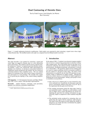
Dual Contouring of Hermite DataTao Ju, Frank Losasso, Scott Schaefer, Joe WarrenRice University Figure 1: A temple undergoing destructive modifications. Both models were generated by dual contouring a signed octree whose edgescontain Hermite data. The modified model on the right was computed from the lefthand model in real-time.Abstract1This paper describes a new method for contouring a signed gridwhose edges are tagged by Hermite data (i.e; exact intersectionpoints and normals). This method avoids the need to explicitly identify and process “features” as required in previous Hermite contouring methods. Using a new, numerically stable representation forquadratic error functions, we develop an octree-based method forsimplifying contours produced by this method. We next extend ourcontouring method to these simplified octrees. This new methodimposes no constraints on the octree (such as being a restricted octree) and requires no “crack patching”. We conclude with a simpletest for preserving the topology of the contour during simplification.In the spring of 2001, 17 students in an advanced computer graphicsclass set out on a semester-long group project to develop a cuttingedge computer game. One of the primary goals for the game was toincorporate technology that allowed real-time modification of thegame geometry. (In gaming terminology, such geometry is referredto as “destructible”.) The geometric engine for the resulting gamewas based on implicit modeling with the environment modeled asthe zero contour of a 3D grid of scalar values. Our choice of thisrepresentation was guided by the fact that CSG operations are particularly simple to implement for implicit models. Although thisgame was a relative success, we noted that our implicit approach tomodeling had several disadvantages. During a post-project review,we identified several problems:CR Categories: I.3.5 [Computation Geometry and Object Modeling]: CSG—Curve, surface, solid and object representationsKeywords:implicit functions, contouring, crack prevention,quadratic error functions, polyhedral simplification troduction Due to the use of a uniform grid, we were restricted to relatively small grid sizes. In particular, the final game could onlyprocess environments defined using grids of size 643 due tothe requirement that the game run in real-time. The resulting environment lacked the sharp edges found inmost polyhedral models. Although we could simulate a smallclass of shapes such as rooms and hallways by cleverly manipulating the sign field, the resulting environment was geometrically simple in comparison to those modeled using BSPtrees. The polyhedral meshes produced by contouring often contained large flat regions tiled by numerous small polygons.The tiling of these flat regions trivially inflated the number ofpolygons in our model and often overwhelmed the graphicscard used for the game.
In preparation for the next version of the gaming class, the instructor and three members of the class (the authors) decided to pursue a yearlong project to rewrite the game engine to address thesedeficiencies. In particular, we focused on adapting three pieces ofrecently developed modeling technology for our program. Each ofthese pieces addresses one of the problems: First, we use an octree in place of a 3D uniform grid. In particular, our octree is inspired by those used in Adaptive DistanceFields [Frisken et al. 2000; Perry and Frisken 2001] in whichsigns are maintained at corners of cubes in the octree. At the leaves of the octree, we tag those edges with signchanges by exact intersection points and their normals fromthe contour. This choice is inspired by the Extended Marching Cubes method of [Kobbelt et al. 2001]. Adding normalsallows this method to exactly reproduce a wide class of polyhedral shapes as well as curved or sharp edges on the contour. Third, we use these normals to define a quadratic error function (QEF) for each leaf of the octree. These QEFs are thenused in an octree-based polyhedral simplification method similar to that of [Lindstrom 2000]. Our method uses the addedinformation specified by the signs attached to the corners ofcubes in the octree to preserve the topology of this contourduring simplification.The resulting representation is an octree whose leaf cubes havesigns at their corners with exact intersections and normals taggingedges that exhibit sign changes. (See the upper left portion of figure2 for an example). Interior nodes in the octree contain QEFs usedduring simplification. This representation can accurately approximate implicit shapes as well as parametric shapes such as subdivision surfaces. (These parametric shapes are imported as polygonalapproximations and scan converted into a signed octree.) The adaptive structure of the octree allows for real-time approximate CSGoperations and simplification of the resulting shapes.Given that we are building on several pieces of previous work,we should make clear our original contributions in this paper. First,we propose a new method for contouring a 3D grid of Hermitedata that avoids the need to explicitly identify and process featuresas done in the Extended Marching Cubes method. After extending this contouring method to the case of multiple materials, wedemonstrate how to model textured contours. We also introduce anew, numerically stable representation for quadratic error functionsthat we use in a standard octree-based method for simplifying thesecontours and their textured regions. We then develop a version ofour contouring method for simplified octrees that imposes no constraints on the octree (such as being a restricted octree) and requiresno crack patching. We conclude with a simple new test for preserving the topology of both the contour and its textured regions duringsimplification.2Dual contouring on uniform gridsAlthough our ultimate goal is to develop a simple contouringmethod that is suitable for octrees, we first consider various methods for contouring signed uniform grids. The upper left portion offigure 2 shows a typical example of a signed uniform grid. Thoseedges of the grid that exhibit a sign change are tagged by Hermitedata consisting of exact intersection points and normals from thecontour. This Hermite data can be computed directly from the implicit definition of the contour or by scan converting a closed polygonal mesh.Figure 2: A signed grid with edges tagged by Hermite data (upper left), its Marching Cubes contour (upper right), its ExtendedMarching Cubes contour (lower left), and its dual contour (lowerright).2.1Previous contouring methodsCube-based methods such as the Marching Cubes (MC) algorithmand its variants generate one or more polygons for each cube in thegrid that intersects the contour. Typically, these methods generateone polygon for each portion of the contour that intersects a particular cube with the vertices of these polygons being positioned at theintersection of the contour with the edges of the cube. The upperright portion of figure 2 shows a 2D example of the MC contourgenerated from the signed grid to its left. The left-hand side of figure 3 shows a 3D example of a sphere generated as the zero contourof the function f [x, y, z] 1 x2 y2 z2 . This contour consistsof a collection of polygons that approximate the restriction of thecontour to individual cubes in the grid.Dual methods such as the SurfaceNets algorithm of [Gibson1998] generate one vertex lying on or near the contour for each cubethat intersects the contour. For each edge in the grid that exhibitsa sign change, the vertices associated with the four cubes that contain the edge are joined to form a quad. The result is a continuouspolygonal surface that approximates the contour. The right-handside of figure 3 shows an example of the same sphere contouredusing the SurfaceNets method. Note that the polygonal mesh produced by the SurfaceNets method is dual to the mesh produced byMC in the standard topological sense: vertices of the SurfaceNetsmesh correspond to faces of the MC mesh and vice versa. Dualmethods typically deliver polygonal meshes with better aspect ratios since the vertices of the mesh are free to move inside the cubeas opposed to being restricted to edges of the grid as in cube-basedmethods. 11 Note that other methods such as [Wood et al. 2000] contour withoutrespect to the underlying fine grid. We focus our attention on grid-based
Figure 3: A sphere contoured using the Marching Cubes method(left) and the SurfaceNets method (right).The Extended Marching Cubes (EMC) method is a hybrid between a cube-based method and a dual method. The EMC methoddetects the presence of sharp features inside a cube by examiningnormals associated with the intersection points on the edges of thecube. Those cubes whose normals lie inside a user-specified coneare deemed to be featureless. In this case, the EMC method generates a polygon(s) using standard MC. For those cubes that docontain a feature, the method generates a vertex positioned at theminimizer of the quadratic functionE[x] (ni · (x pi ))2(1)iwhere the pairs pi , ni correspond to the intersections (and unit normals) of the contour with the edges of the cube. Once this vertex hasbeen positioned, the method generates a triangle fan to the edges onthe boundary of the cube. Finally, if two adjacent cubes both contain feature vertices, then the pair of triangles generated by the fanto their common face has its common edge flipped to form a featureedge. The lower left portion of figure 2 shows a 2D example of thecontour generated by EMC.Figure 4: A mechanical part generated by dual contouring Hermitedata on a 643 grid.for positioning vertices on the contour.) By using QEFs to positionall of the vertices of the contour, this method avoids the need toexplicit test for features. Vertices on the contour are simply positioned to be consistent with the normals associated with the data.The lower right portion of figure 2 shows a 2D example of the dualcontour generated by the Hermite data in the upper left portion ofthe figure.Figure 4 shows a 3D example of a mechanical part modeled bydual contouring Hermite data on a 643 grid. The left image showsa smooth shaded version of the part while the right image showsthe polygonal mesh produced by dual contouring. The intersectionpoints and normals for the model were generated from a closedsubdivision surface. A sign field denoting the inside/outside of themodel was computed using a standard scan conversion algorithm asdescribed in [Foley et al. 1995].2.32.2Dual contouring of Hermite dataThe main advantage of the EMC method is that it uses Hermitedata and QEFs in positioning the vertices associated with cubesthat contain features. This Hermite approach can generate contoursthat contain both sharp vertices and sharp edges. One drawback ofthis method is the need to explicitly test for such features and tothen perform some type of special processing in these cases. Asan alternative to the EMC method, we propose the following dualcontouring method for Hermite data:1. For each cube that exhibits a sign change, generate a vertexpositioned at the minimizer of the quadratic function of equation 1.2. For each edge that exhibits a sign change, generate a quadconnecting the minimizing vertices of the four cubes containing the edge.This method is an interesting hybrid of the EMC method andthe SurfaceNets method. It uses the EMC method’s feature vertex rule for positioning all vertices of the contour while using theSurfaceNets method to determine the connectivity of these vertices.(Note that the SurfaceNets method uses a completely different rulemethods like the ones above since this grid structure is the basis of our fastCSG operations.Representing and minimizing QEFsAt this point, we should make a few comments concerning how werepresent and minimize quadratic error functions. The function E[x]of equation 1 is constructed from a collection of intersection pointspi and normals ni . This function E[x] can be expressed as the innerproduct (Ax b)T (Ax b) where A is a matrix whose rows are thenormals ni and b is a vector whose entries are ni · pi . Typically, thequadratic function E[x] is expanded into the formE[x] xT AT Ax 2xT AT b bT b(2)where the matrix AT A is a symmetric 3 3 matrix, AT b is a columnvector of length three and bT b is a scalar. The advantage of this expansion is that only the matrices AT A, AT b and bT b need be stored(10 floats), as opposed to storing the matrices A and b. Furthermore, a minimizing value x̂ for E[x] can be computed by solvingthe normal equations AT Ax̂ AT b.One drawback of this representation is that it is numerically unstable. For example, consider computing the value of E[x] in floating point arithmetic when the intersection points and normals usedin constructing E[x] are sampled from a flat area. For a grid of size2563 (as in figure 1), the magnitude of bT b can be on the order of106 . Since floats are only accurate to six decimal digits, if E[x] isevaluated at points on the original flat area (where E[x] should bezero), the resulting value has an error on the order of 1.One possible solution to this problem is to use double precisionnumbers instead of floats in representing AT A, AT b and bT b. Us-
ing doubles, the value of E[x] in our flat example now has an errorof 10 6 . Of course, the main drawback of using doubles in placeof floats is that the space require to store a QEF is doubled. Forour application, we found this solution to be problematic since ourprogram tended to be space bound as opposed to being time bound.(See the last section for details.)An alternative representation for QEFs that delivers the accuracyof doubles while using only floats is based on the QR decomposition [Golub and Van Loan 1989]. If (A b) is the matrix formed byappending the column vector b to the matrix A, the idea behind thisdecomposition is to compute an orthogonal matrix Q whose productwith (A b) is an upper triangular matrix of the form xxxx 0xxx  b̂ 0xx 0 0r .(3) 00x 00 0 0000 . . . . .Here,  is an upper triangular 3 3 matrix, b̂ is a column vectorof length 3 and r is a scalar. This matrix Q can be expressed asthe product of a sequence of Givens rotations where each rotationzeroes a single entry in the lower part of (A b).Since any orthogonal matrix Q satisfies the relation QT Q I,E[x] can be rewritten as(Ax b)T (Ax b) (Ax b)T QT Q(Ax b) (QAx Qb)T (QAx Qb) (Âx b̂)T (Âx b̂) r2To evaluate E[x] in this form, we compute the product of the vectorÂx b̂ with itself and then add r 2 . Returning to our previous flatexample, we note that b has entries on the order of 103 and thereforeÂx b̂ has entries that are on the order of 10 3 when x is chosenfrom the flat regions. Therefore, the computed value of E[x] will beon the order of 10 6 .If  is non-singular, the minimizing x̂ can be computed by solving Âx̂ b̂ using back substitution. However, during dual contouring,  is often computed from noisy normals that are nearlycoplanar. In this case, the matrix  is nearly singular. As a result,the minimizing x̂ may lie far outside the defining cube. To solvethis problem, we compute the SVD decomposition of  and formits pseudo-inverse by truncating its small singular values as donein [Kobbelt et al. 2001; Lindstrom 2000]. Based on experimentation, we typically truncate those singular values with a magnitudeof less than 0.1. Using the resulting pseudo-inverse, we then approximately solve Âx̂ b̂ while minimizing the distance of x̂ to thecentroid of the intersection points pi .2.4Modeling textured contoursIn figure 3, both contouring algorithms produced surfaces thatbounded the transition from negative (empty) space to positive(solid) space. In a realistic environment, solids are not composed ofa single homogeneous material. In practice, solids are composed ofa collection of materials; each of which induces a region with a distinct texture on the contour. Figure 5 shows an example of a cubeconsisting of two materials, a gold material formed by extruding aChinese character through the cube and a red material forming theremaining portion of the cube. Note that the gold material is a truesolid (and not a surface texture) since the gold character extends allthe way through the cube (as evidenced by the cube after a sphericalcut on the right).This partition of solids into distinct materials can be modeledimplicitly by replacing the signs and (corresponding to emptyFigure 5: A solid cube undergoing a sequence of CSG operations.Figure 6: The dual contour for a three-index grid (left), treating thetwo solid (dark) indices as single index(right)and solid space) by a material index. In this representation, eachgrid point has an index corresponding to a distinct material.(See[Bloomenthal and Ferguson 1995; Bonnell et al. 2000] for examples of similar approaches.) Figure 6 shows a 2D grid with threedistinct indices; the gray and black grid points denote distinct solidmaterials while white grid points denote empty space. As before,edges that exhibit index changes are also tagged by exact intersection points and normals. During contouring, this Hermite data isused in equation 1 to define a QEF associated with each cube in thegrid. Next, for each edge that exhibits an index change, dual contouring generates a quad connecting the minimizers of the QEFsfor the four cubes containing the edge. The left portion of figure 6shows the dual contour that separates the three materials.If the viewer is restricted to empty space, we can optimize thiscontouring method for solids that consist of several different materials. In particular, quads generated by solid/solid edges are notvisible from empty space. The remaining quads correspond tosolid/empty edges and can be textured using the material properties of the solid endpoint of the edge 2 . In figure 5, the underlyinggrid contains three materials: empty space, gold material, and redmaterial. The resulting dual contour consists of red quads generated by red/empty edges and gold quads generated by gold/emptyedges. Red/gold edges do not generate quads.2 Each material has an associated “black box” defined during the material’s addition to the model that converts 3D geometric coordinates into 2Dtexture coordinates.
When three or more materials meet inside a single cube, dualcontouring places the minimizing vertex at or near their intersectionpoint. This positioning allows the outlines of letters and charactersembossed on a surface to be reproduced very accurately. (The righthand portion of figure 12 shows a close-up example of this effect.)Cube-based contouring methods constrain the vertices of the contour to lie on the edges of the 3D grid making this effect difficult toachieve.The move to the multi-material case allows for several interesting variations on the CSG operations used in the two-material case.In place of the standard CSG operations, we use a single operationAdd that overwrites a portion of the existing model with a new material. Subtractive operations such as the spherical cut in the upperright of figure 5 can be represented as adding a sphere of emptyspace to the model. Another useful variant of Add is the operationReplace that overwrites only the solid portion of the model. Thisoperation can also be used to simulate texturing a portion of thecontour. For example, the lower images in figure 5 show a portionof the solid replaced by a blue material and then subsequently cutby a sphere.3Figure 7: Closeups of two polygonal approximations to the templecomputed using the standard (left) and QR (right) representation forQEFs.The only modification that we make to this method is to changeour internal representation for QEFs to take advantage of the QRdecomposition discussed in the previous section. To this end, werepresent a QEF in terms of 10 floats corresponding to the entriesof the upper triangular matrix of equation 3. Adding two QEFs corresponds to merging the rows of their two upper triangular matricesto form a single 8 4 matrix of the formx 0 0 0 x 0 00 Adaptive dual contouringThe previous algorithm for dual contouring has the obvious disadvantage of being formulated for uniform grids. In practice, most ofa uniform grid is devoted to storing homogeneous cubes (i.e; cubeswhose vertices all have the same sign). Only a small fraction of thecubes are heterogeneous and, thus, intersect the contour. One wayto avoid this waste of space is to replace the uniform grid by anoctree. In this section, we describe an adaptive version of dual contouring based on simplifying an octree whose leaves contain QEFs.This method is essentially an adaptive variant of a uniform simplification method due to [Lindstrom 2000]. Our method has threesteps: Generate a signed octree whose homogeneous leaves are maximally collapsed. Construct a QEF for each heterogeneous leaf and simplify theoctree using these QEFs. Recursively generate polygons for this simplified octree.Note that our method also differs from Lindstrom’s method in thatwe generate polygons from the signed octree instead of collapsingpolygons in an existing mesh.Generating the signed octree in the first step is relatively straightforward. For implicit or polygonal models, this octree can be constructed recursively in a top-down manner by spatially partitioningthe models. For signed data on a uniform grid, this octree can begenerated in a bottom-up manner by recursively collapsing homogeneous regions. The next two subsections examine the second andthird parts of this process in more detail. (Note that the adaptivemethod described here works for the multi-material case withoutmodification.)3.1Octree simplification using QEFsOur approach to the second step of the adaptive method is to construct a QEF associated with each heterogeneous leaf using equation 1. Note that the residual associated with the minimizer of thisQEF estimates how well the minimizing vertex approximates theoriginal geometry [Garland and Heckbert 1998]. Our approach tosimplifying the resulting octree is to form QEFs at interior nodesof the octree by adding the QEFs associated with the leaves of thesubtree rooted by the node. Those interior nodes whose QEFs havea residual less than a given tolerance are collapsed into leaves.xx00xx00xxx0xxx0 xx x x x x xxand then performing a sequence of Givens rotations to bring thematrix back into upper triangular form of equation 3. Due to the orthogonality of the Givens rotations, the QEF for the merged systemis the sum of QEFs associated with the unmerged systems. Notethat bringing the merged system back into upper triangular formis slower (around 150 arithmetic operations) than simply adding10 floats as done in the standard representation. However, the improved stability of the representation leads to better simplifications.Figure 7 gives a concrete illustration of the advantage of the QRrepresentation’s stability. The meshes in this figure show two simplifications of the temple from figure 1 to an error of 0.014; the leftmesh was computed using the standard representation for QEFs, theright mesh was computed using the QR representation for QEFs.(To give a sense of scale, the temple was defined over a 2563 unitgrid.) Due to the numerical error introduced by the instability of thestandard representation, the mesh on the left contains 78K polygonswhile the mesh on the right has 36K polygons.3.2Polygon generation for simplified octreesGiven this simplified octree, our next task is to modify the polygon generation phase of dual contouring appropriately. For cubebased methods, this problem of generating contours from octreeshas been extensively studied [Bloomenthal 1988; Wilhelms andGelder 1992; Livnat et al. 1996; Shekhar et al. 1996; Westermannet al. 1999; Frisken et al. 2000; Cignoni et al. 2000]. Typically,these methods restrict the octree to have neighboring leaves thatdiffer by at most one level (i.e; “restricted” octrees) and usually perform some type of crack repair to ensure a closed contour. [Perryand Frisken 2001] describes a variant of the SurfaceNets algorithmfor signed octrees based on enumerating the edges associated withleaves of the octree. In particular, For each edge that exhibits a sign change, generate all triangles that connect the vertices associated with any three distinctcubes containing the edge.
Figure 9: Recursive functions faceProc (black) and edgeProc(gray) used in enumerating pairs of leaf squares that contain a common edge.Figure 8: Three simplified versions of the mechanical part.To avoid generating redundant triangles, this method culls someof the generated triangles based on the relative positions of theircorresponding edges inside a leaf cube. In the final mesh, each edgecorresponds to either one or two triangles (a quad) on the resultingcontour. The main disadvantage of this method (as acknowledgedby the authors) is that it occasionally yields contours with cracks.The authors identify these problem configurations and avoid themby performing extra subdivision on the octree.We propose a simpler rule for dual contouring signed octreesthat avoids this need for extra subdivision. The rule is based on theobservation that only those edges of leaf cubes that do not properlycontain an edge of a neighboring leaf should generate a polygon.We refer to such edges as the minimal edges of the octree. Thus,our rule for polygon generation is For each minimal edge that exhibits a sign change, generatea polygon connecting the minimizing vertices of cubes thatcontain the edge.This rule has the property that it always produces a closed polygonal mesh for any simplified octree. In particular, every edge inthe mesh is contained by an even number of polygons. To provethis fact, we observe that edges in the dual contour are generatedby pairs of face-adjacent leaf cubes. The minimal edges tiling theboundary of their common square face always exhibit an even number of sign changes since the boundary of the square is a closedcurve. Therefore, the rule always generates an even number of polygons containing the edge. For example, the common square facealways consists of four consecutive edges in the uniform case. Thischain of four edges can exhibit either two or four sign changes andconsequently generate two or four polygons containing the common edge. (It is possible to construct signed octrees that generatedual contours with 6 or more polygons share a common edge.) Figure 8 shows three simplified approximations to the mechanical part.Note that the rightmost mesh has undergone a topology change.This rule generates triangles instead of quads in transitional areasof the octree where a single coarse cube is face-adjacent to four finecubes. Minimal edges in the middle of the shared coarse face arecontained by only three cubes and generate triangles that form atransition between coarse quads and fine quads. Figure 7 showsmany examples of such transition triangles produced by contouringa simplified octree.Note that the Perry/Frisken rule enumerates edges in the octreeand then locates those cubes that contain the edge. This neighborfinding entails either walking up and down the octree or explicitlymaintaining links between neighboring cubes. Instead of enumerating edges and trying to find neighbors, we propose a recursivemethod for enumerating those sets of cubes that contain a commonminimal edge. For the sake of simplicity, we explain this enumeration method for quadtrees while noting that a similar method worksfor octrees.The key to this enumeration procedure are two recursive functions faceProc[q] and edgeProc[q1 ,q2 ]. Given an interior nodeq in the quadtree, faceProc[q] recursively calls itself on the fourchildren of q as well as calling edgeProc on all four pairs of edgeadjacent children of q. Given a pair of edge-adjacent interior nodesq1 and q2 , edgeProc[q1 ,q2 ] recursively calls itself on the twopairs of edge-adjacent children spanning the common edge betweenq1 and q2 . Figure 9 depicts the mutually recursive structure of thesetwo functions.The recursive calls to edgeProc[q1 ,q2 ] terminate when bothq1 and q2 are leaves of the quadtree. At this point, the call toedgeProc has all of the information necessary to generate the segment associated with the minimal edge shared by q1 and q2 . Notethe running time of this method is linear in the size of the quadtreesince there is one call to faceProc for each square in the quadtreeand one call to edgeProc for each edge in the quadtree.Contouring octrees requires three functions cellProc[q] ,faceProc[q1 ,q2 ] and edgeProc[q1 ,q2 ,q3 ,q4 ] . The function cellProc spawns eight calls to cellProc, twelve callsto faceProc and six calls to edgeProc. faceProc spawnsfour calls to faceProc and four calls to edgeProc. Finally,edgeProc spawns two calls to edgeProc. The recursive calls toedgeProc[q1 ,q2 ,q3 ,q4 ] terminate at minimal edges of the octrees where all of the qi ’s are leaves.4Simplification with topology safetySimplification methods such as [Rossignac and Borrell 1993; Lindstrom 2000] have the property that the topological connectivity ofthe polygonal mesh may change during simplification. More sophisticated methods such as [Stander and Hart 1997; Gerstner andPajarola 2000; Wood et al. 2000; Guskov and Wood 2001] weredeveloped to maintain the connectivity of the mesh during simplification. Unfortunately, in our setting, not only can the topological connectivity of the contour change during simplification, butalso the connectivity of its textured regions. The left side of figure 12 shows an example of a simplification in which distinct partsof the Chinese character have merged making it difficult to recognize. While these topological changes are not always undesirable,we wish to have the option of maintaining the topologica
one polygon for each portion of the contour that intersects a partic-ular cube with the vertices of these polygons being positioned at the intersection of the contour with the edges of the cube. The upper right portion of figure 2 shows a 2D example of the MC contour generated from the signed grid to its left. The left-hand side of fig-