Transcription
Confirming PagesChapter4Labor Market EquilibriumOrder is not pressure which is imposed on society from without, but anequilibrium which is set up from within.—José Ortega y GassetWorkers prefer to work when the wage is high, and firms prefer to hire when the wage islow. Labor market equilibrium “balances out” the conflicting desires of workers and firmsand determines the wage and employment observed in the labor market. By understandinghow equilibrium is reached, we can address what is perhaps the most interesting questionin labor economics: Why do wages and employment go up and down?This chapter analyzes the properties of equilibrium in a perfectly competitive labormarket. We will see that if markets are competitive and if firms and workers are free toenter and leave these markets, the equilibrium allocation of workers to firms is efficient;the sorting of workers to firms maximizes the total gains that workers and firms accumulate by trading with each other. This result is an example of Adam Smith’s justly famousinvisible hand theorem, wherein labor market participants in search of their own selfish goals attain an outcome that no one in the market consciously sought to achieve. Theimplication that competitive labor markets are efficient plays an important role in the framing of public policy. In fact, the impact of many government programs is often debated interms of whether the particular policy leads to a more efficient allocation of resources orwhether the efficiency costs are substantial.We also will analyze the properties of labor market equilibrium under alternative marketstructures, such as monopsonies (where there is only one buyer of labor) and monopolies(where there is only one seller of the output). Each of these market structures generates anequilibrium with its own unique features. Monopsonists, for instance, generally hire fewerworkers and pay less than competitive firms.Finally, the chapter uses a number of policy applications—such as taxes, subsidies,and immigration—to illustrate how government policies shift the labor market to a different equilibrium, thereby altering the economic opportunities available to both firms andworkers.144bor23208 ch04 144-202.indd 14427/10/11 10:58 AM
Confirming PagesLabor Market Equilibrium4-1145Equilibrium in a Single Competitive Labor MarketWe have already briefly discussed how a competitive labor market attains equilibrium. Wenow provide a more detailed discussion of the properties of this equilibrium. Figure 4-1 illustrates the familiar graph showing the intersection of labor supply (S) and labor demand (D)curves in a competitive market. The supply curve gives the total number of employeehours that agents in the economy allocate to the market at any given wage level; thedemand curve gives the total number of employee-hours that firms in the market demandat that wage. Equilibrium occurs when supply equals demand, generating the competitivewage w* and employment E*. The wage w* is the market-clearing wage because any otherwage level would create either upward or downward pressures on the wage; there wouldbe too many jobs chasing the few available workers or too many workers competing forthe few available jobs.Once the competitive wage level is determined in this fashion, each firm in this industryhires workers up to the point where the value of marginal product of labor equals the competitive wage. The first firm hires E1 workers; the second firm hires E2 workers; and so on.The total number of workers hired by all the firms in the industry must equal the market’sequilibrium employment level, E*.FIGURE 4-1 Equilibrium in a Competitive Labor MarketThe labor market is in equilibrium when supply equals demand; E* workers are employed at a wage of w*. In equilibrium,all persons who are looking for work at the going wage can find a job. The triangle P gives the producer surplus; thetriangle Q gives the worker surplus. A competitive market maximizes the gains from trade, or the sum P Q.DollarsSPw*QDELbor23208 ch04 144-202.indd 145E*EHEmployment27/10/11 10:58 AM
Confirming PagesTheory at WorkTHE INTIFADAH AND PALESTINIAN WAGESThroughout much of the 1980s, nearly 110,000 Palestinians who resided in the occupied West Bank and GazaStrip commuted to Israel for their jobs. Many of thesePalestinians were employed in the construction or agriculture industries.As a result of the Intifadah—the Palestinian uprisingagainst Israeli control of the West Bank and Gaza territories that began in 1988—there were major disruptionsin the flow of these workers into Israel. Israeli authorities,for instance, stepped up spot checks of work permits andbegan to enforce the ban on Palestinians spending thenight in Israel, while strikes and curfews in the occupied territories limited the mobility of commuting workers. Withinone year, the daily absenteeism rate jumped from less than2 percent to more than 30 percent; the average numberof work days in a month dropped from 22 to 17; and thelength of time it took a commuting Palestinian to reach thework location rose from 30 minutes to three or four hours.The Intifadah, therefore, greatly reduced the supply of Palestinian commuters in Israel. The supply anddemand framework suggests that the uprising shouldhave increased the equilibrium wages of these Palestinian workers. In fact, this is what occurred. The roughly50 percent cut in the labor supply of Palestinian commuters increased their real wage by about 50 percent,implying that the demand elasticity for Palestinian commuters is on the order of 1.Source: Joshua D. Angrist, “Short-Run Demand for PalestinianLabor,” Journal of Labor Economics 14 (July 1996): 425–453.As Figure 4-1 shows, there is no unemployment in a competitive labor market. At themarket wage w*, the number of persons who want to work equals the number of workersfirms want to hire. Persons who are not working are also not looking for work at the goingwage. Of course, many of these persons would enter the labor market if the wage rose (andmany would withdraw if the wage fell).Needless to say, a modern industrialized economy is continually subjected to many shocksthat shift both the supply and demand curves. It is unlikely, therefore, that the labor marketactually ever reaches a stable equilibrium—with wages and employment remaining at a constant level for a long time. Nevertheless, the concept of labor market equilibrium remainsuseful because it helps us understand why wages and employment seem to go up or downin response to particular economic or political events. As the labor market reacts to a particular shock, wages and employment will tend to move toward their new equilibrium level.EfficiencyFigure 4-1 also shows the benefits that accrue to the national economy as workers andfirms trade with each other in the labor market. In a competitive market, E* workers areemployed at a wage of w*. The total revenue accruing to the firm can be easily calculatedby adding up the value of marginal product of the first worker, the second worker, and allworkers up to E*. This sum, in effect, gives the value of the total product produced by allworkers in a competitive equilibrium. Because the labor demand curve gives the value ofmarginal product, it must be the case that the area under the labor demand curve gives thevalue of total product. Each worker receives a wage of w*. Hence, the profits accruing tofirms, which we call producer surplus, are given by the area of the triangle P.11146bor23208 ch04 144-202.indd 146To simplify the discussion, assume that labor is the only factor in the production function.27/10/11 10:58 AM
Confirming PagesLabor Market Equilibrium147Workers also gain. The supply curve gives the wage required to bribe additional workers into the labor market. In effect, the height of the supply curve at a given point measures the value of the marginal worker’s time in alternative uses. The difference betweenwhat the worker receives (that is, the competitive wage w*) and the value of the worker’stime outside the labor market gives the gains accruing to workers. This quantity is calledworker surplus and is given by the area of the triangle Q in Figure 4-1.The total gains from trade accruing to the national economy are given by the sum ofproducer surplus and worker surplus, or the area P Q. The competitive market maximizesthe total gains from trade accruing to the economy. To see why, consider what the gainswould be if firms hired more than E* workers, say EH. The “excess” workers have a valueof marginal product that is less than their value of time elsewhere. In effect, these workersare not being efficiently used by the labor market; they are better off elsewhere. Similarly, consider what would happen if firms hired too few workers, say EL. The “missing”workers have a value of marginal product that exceeds their value of time elsewhere, andtheir resources would be more efficiently used if they worked.The allocation of persons to firms that maximizes the total gains from trade in the labormarket is called an efficient allocation. A competitive equilibrium generates an efficientallocation of labor resources.4-2Competitive Equilibrium across Labor MarketsThe discussion in the previous section focused on the consequences of equilibrium in asingle competitive labor market. The economy, however, typically consists of many labormarkets, even for workers who have similar skills. These labor markets might be differentiated by region (so that we can talk about the labor market in the Northeast and the labormarket in California), or by industry (the labor market for production workers in the automobile industry and the labor market for production workers in the steel industry).Suppose there are two regional labor markets in the economy, the North and the South.We assume that the two markets employ workers of similar skills so that persons workingin the North are perfect substitutes for persons working in the South. Figure 4-2 illustratesthe labor supply and labor demand curves in each of the two labor markets (SN and DN inthe North, and SS and DS in the South). For simplicity, the supply curves are represented byvertical lines, implying that supply is perfectly inelastic within each region. As drawn, theequilibrium wage in the North, wN, exceeds the equilibrium wage in the South, wS.Can this wage differential between the two regions persist and represent a true competitive equilibrium? No. After all, workers in the South see their northern counterparts earning more. This wage differential encourages southern workers to pack up and move north,where they can earn higher wages and presumably attain a higher level of utility. Employersin the North also see the wage differential and realize that they can do better by movingto the South. After all, workers are equally skilled in the two regions, and firms can makemore money by hiring cheaper labor.If workers can move across regions freely, the migration flow will shift the supply curves inboth regions. In the South, the supply curve for labor would shift to the left (to S S) as southernworkers leave the region, raising the southern wage. In the North, the supply curve would shiftto the right (to S N) as the southerners arrived, depressing the northern wage. If there were freebor23208 ch04 144-202.indd 14727/10/11 10:58 AM
Confirming Pages148Chapter 4FIGURE 4-2 Competitive Equilibrium in Two Labor Markets Linked by MigrationThe wage in the northern region (wN) exceeds the wage in the southern region (wS). Southern workers want to movenorth, shifting the southern supply curve to the left and the northern supply curve to the right. In the end, wages areequated across regions (at w*). The migration of workers reduces the gains from trade in the South by the size of theshaded trapezoid in the southern labor market, and increases the gains from trade in the North by the size of the largershaded trapezoid in the northern labor market. Migration increases the total gains from trade in the national economyby the triangle mentEmployment(a) The Northern Labor Market(b) The Southern Labor Marketentry and exit of workers in and out of labor markets, the national economy would eventuallybe characterized by a single wage, w*.Note that wages across the two labor markets also would be equalized if firms (instead ofworkers) could freely enter and exit labor markets. When northern firms close their plantsand move to the South, the demand curve for northern labor shifts to the left and lowers thenorthern wage, whereas the demand curve for southern labor shifts to the right, raising thesouthern wage. The incentives for firms to move across markets evaporate once the regionalwage differential disappears. As long as either workers or firms are free to enter and exitlabor markets, therefore, a competitive economy will be characterized by a single wage.2Efficiency RevisitedThe “single wage” property of a competitive equilibrium has important implications foreconomic efficiency. Recall that, in a competitive equilibrium, the wage equals the valueof marginal product of labor. As firms and workers move to the region that provides the2A study of whether a labor market can be considered competitive is given by Stephen Machin andAlan Manning, “A Test of Competitive Labor Market Theory: The Wage Structure among Care Assistants in the South of England,” Industrial and Labor Relations Review 57 (April 2004): 371–385.bor23208 ch04 144-202.indd 14827/10/11 10:58 AM
Confirming PagesLabor Market Equilibrium149best opportunities, they eliminate regional wage differentials. Therefore, workers of givenskills have the same value of marginal product of labor in all markets.The allocation of workers to firms that equates the value of marginal product acrossmarkets is also the sorting that leads to an efficient allocation of labor resources. To seewhy, suppose that a benevolent dictator takes over the economy and that this dictator hasthe power to dispatch workers across regions. In making allocation decisions, suppose thisbenevolent dictator has one overriding objective: to allocate workers to those places wherethey are most productive. When the dictator first takes over, he faces the initial situationillustrated in Figure 4-2, where the competitive wage in the North (wN) exceeds the competitive wage in the South (wS). Note that this wage gap implies that the value of marginalproduct of labor is greater in the North than in the South.The dictator picks a worker in the South at random. What should he do with this worker?Because the dictator wants to place this worker where he is most productive, the worker isdispatched to the North. In fact, the dictator will keep reallocating workers to the northernregion as long as the value of marginal product of labor is greater in the North than in theSouth. The law of diminishing returns implies that as the dictator forces more and morepeople to work in the North, the value of marginal product of northern workers declinesand the value of marginal product of southern workers rises. The dictator will stop reallocating persons when the labor force consists only of persons whose value of marginalproduct exceeds the value of their time outside the labor market and when the value ofmarginal product is the same in all labor markets.It is also easy to see how migration leads to an efficient allocation of resources by calculating the gains from trade in the labor market. Because the supply curves in Figure 4-2are perfectly inelastic (implying that the value of time outside the labor market is zero), thetotal gains from trade are given by the area under the demand curve up to the equilibriumlevel of employment. The migration of workers out of the South reduces the total gainsfrom trade in the South by the shaded area of the trapezoid in the southern labor market.The migration of workers into the North increases the total gains from trade in the Northby the shaded area of the trapezoid in the northern labor market. A comparison of the twotrapezoids reveals that the area of the northern trapezoid exceeds the area of the southerntrapezoid by the size of the triangle ABC, implying that the total gains from trade in thenational economy increase as a result of worker migration.The surprising implication of our analysis should be clear: Through an “invisiblehand,” workers and firms that search selfishly for better opportunities accomplish a goalthat no one in the economy had in mind: an efficient allocation of resources.Convergence of Regional Wage LevelsThere is a great deal of interest in determining whether regional wage differentials in theUnited States (as well as in other countries) narrow over time, as implied by our analysis oflabor market equilibrium. Many empirical studies suggest that there is indeed a tendencytoward convergence.33Robert J. Barro and Xavier Sala-i-Martin, “Convergence across States and Regions,” Brookings Paperson Economic Activity (1991): 107–158; and Olivier Jean Blanchard and Lawrence F. Katz, “RegionalEvolutions,” Brookings Papers on Economic Activity 1 (1992): 1–61.bor23208 ch04 144-202.indd 14927/10/11 10:58 AM
Confirming Pages150Chapter 4FIGURE 4-3 Wage Convergence across StatesSource: Olivier Jean Blanchard and Lawrence F. Katz, “Regional Evolutions,” Brookings Papers on Economic Activity 1 (1992): 1–61.5.7LAGA5.5MSPercent Annual Wage GrowthAR5.3ME TXMO PA WIINIL COUTNYKYAZMT uring Wage in 1950Figure 4-3 summarizes the key data underlying the study of wage convergence acrossstates in the United States. The figure relates the annual growth rate in the state’s manufacturing wage between 1950 and 1990 to the initial wage level in 1950. There is a strongnegative relationship between the rate of wage growth and the initial wage level so that thestates with the lowest wages in 1950 subsequently experienced the fastest wage growth. Ithas been estimated that about half the wage gap across states disappears in about 30 years.The evidence indicates, therefore, that wage levels do converge over time—although itmay take a few decades before wages are equalized across markets.Wage convergence also is found in countries where the workforce is less mobile, suchas Japan. A study of the Japanese labor market indicates that wage differentials acrossprefectures (a geographic unit roughly comparable to a large U.S. county) disappear atabout the same rate as interstate wage differentials in the United States: half of the regionaldifferences vanish within a generation.44Robert J. Barro and Xavier Sala-i-Martin, “Regional Growth and Migration: A Japan–United StatesComparison,” Journal of the Japanese and International Economies 6 (December 1992): 312–346.Other international studies of wage convergence within regions of a country include Christer Lundh,Lennart Schon, and Lars Svensson, “Regional Wages in Industry and Labour Market Integration inSweden, 1861–1913,” Scandinavian Economic History Review 53 (2005): 71–84; and Joan R. Roses andBlanca Sanchez-Alonso, “Regional Wage Convergence in Spain 1850–1930,” Explorations in EconomicHistory 41 (October 2004): 404–425.bor23208 ch04 144-202.indd 15027/10/11 10:58 AM
Confirming Pages151Labor Market EquilibriumOf course, the efficient allocation of workers across labor markets and the resultingwage convergence are not limited to labor markets within a country, but also might occurwhen we compare labor markets across countries. Many recent studies have attempted todetermine if international differences in per capita income are narrowing.5 Much of thiswork is motivated by a desire to understand why the income gap between rich and poorcountries seems to persist.The empirical studies typically conclude that when one compares two countries withroughly similar endowments of human capital (for example, the educational attainmentof the population), the wage gap between these countries narrows over time, with abouthalf the gap disappearing within a generation. This result, called “conditional” convergence (because it compares countries that are already similar in terms of the human capitalendowment of the workforce), does not necessarily imply that there will be convergencein income levels between rich and poor countries. The wage gap between rich and poorcountries can persist for much longer periods because the very low levels of human capital in poor countries do not permit these countries to be on the same growth path as thewealthier countries.The rate of convergence in income levels across countries plays an important role inthe debate over many crucial policy issues. Consider, for instance, the long-term effects ofthe North American Free Trade Agreement (NAFTA). This agreement permits the unhampered transportation of goods (but not of people) across international boundaries throughout much of the North American continent (Canada, the United States, and Mexico).In 2000, per capita GDP in the United States was over three times as large as that inMexico. Our analysis suggests that NAFTA should eventually reduce the huge incomedifferential between Mexico and the United States. As U.S. firms move to Mexico to takeadvantage of the cheaper labor, the demand curve for Mexican labor shifts out and thewage differential between the two countries will narrow. Our discussion suggests that U.S.workers who are most substitutable with Mexican workers will experience a wage cut asa result of the increase in trade. At the same time, however, American consumers willgain from the increased availability of cheaper goods. In short, NAFTA will likely create distinct groups of winners and losers in the American economy. In fact, the availableevidence suggests that manufacturing firms are now finding the Mexican labor market tobe relatively expensive.6Although NAFTA inevitably affects the distribution of income across the three countries, our analysis of labor market efficiency implies that the total income of the countriesin the free-trade zone is maximized when economic opportunities are equalized acrosscountries. In other words, the equalization of wages across the three signatories of NAFTAincreases the size of the economic pie available to the entire region. In principle, the additional wealth can be redistributed to the population of the three countries so as to make5Robert J. Barro, “Economic Growth in a Cross-Section of Countries,” Quarterly Journal of Economics105 (May 1990): 501–526; N. Gregory Mankiw, David Romer, and David N. Weil, “A Contributionto the Empirics of Economic Growth,” Quarterly Journal of Economics 107 (May 1991): 407–437;and Xavier Sala-i-Martin, “The World Distribution of Income: Falling Poverty and . . . Convergence,Period,” Quarterly Journal of Economics 121 (May 2006): 351–397.6bor23208 ch04 144-202.indd 151Elisabeth Malkin, “Manufacturing Jobs Are Exiting Mexico,” New York Times, November 5, 2002.27/10/11 10:58 AM
Confirming Pages152Chapter 4everyone in the region better off. This link between free trade and economic efficiency istypically the essential point emphasized by economists when they argue in favor of moreopen markets.74-3Policy Application: Payroll Taxes and SubsidiesWe can easily illustrate the usefulness of the supply and demand framework by considering a government policy that shifts the labor demand curve. In the United States, somegovernment programs are funded partly through a payroll tax assessed on employers. In2011, firms paid a tax of 6.2 percent on the first 106,800 of a worker’s annual earnings tofund the Social Security system and an additional tax of 1.45 percent on all of a worker’sannual earnings to fund Medicare.8 In other countries, the payroll tax on employers is evenhigher. In Germany, for example, the payroll tax is 17.2 percent; in Italy, it is 21.2 percent;and in France, it is 25.3 percent.9What happens to wages and employment when the government assesses a payroll tax onemployers? Figure 4-4 answers this question. Prior to the imposition of the tax, the labordemand curve is given by D0 and the supply of labor to the industry is given by S. In thecompetitive equilibrium given by point A, E0 workers are hired at a wage of w0 dollars.Each point on the demand curve gives the number of workers that employers wish tohire at a particular wage. In particular, employers are willing to hire E0 workers if eachworker costs w0 dollars. To simplify the analysis, consider a very simple form of payrolltax. In particular, the firm will pay a tax of 1 for every employee-hour it hires. In otherwords, if the wage is 10 an hour, the total cost of hiring an hour of labor will be 11 ( 10goes to the worker and 1 goes to the government). Because employers are only willingto pay a total of w0 dollars to hire the E0 workers, the imposition of the payroll tax impliesthat employers are now only willing to pay a wage rate of w0 1 dollars to the workers inorder to hire E0 of them.The payroll tax assessed on employers, therefore, leads to a downward parallel shift inthe labor demand curve to D1, as illustrated in Figure 4-4. The new demand curve reflectsthe wedge that exists between the total amount that employers must pay to hire a workerand the amount that workers actually receive from the employer. In other words, employers take into account the total cost of hiring labor when they make their hiring decisions—so that the amount that they will want to pay to workers has to shift down by 1 in orderto cover the payroll tax. The payroll tax moves the labor market to a new equilibrium(point B in the figure). The number of workers hired declines to E1. The equilibrium wagerate—that is, the wage rate actually received by workers—falls to w1, but the total cost ofhiring a worker rises to w1 1.7A detailed discussion of the impact of trade on labor markets is given by George Johnson and FrankStafford, “The Labor Market Implications of International Trade,” in Orley C. Ashenfelter and DavidCard, editors, Handbook of Labor Economics, vol. 3B, Amsterdam: Elsevier, 1999, pp. 2215–2288.8Workers are also assessed a similar tax on their earnings, so the total tax payment is 15.3 percent onthe first 106,800 of salary, and a 2.9 percent tax on wages above 106,800.9U.S. Bureau of the Census, Statistical Abstract of the United States, 2012. Washington, DC: Government Printing Office, 2011, Table 1361.bor23208 ch04 144-202.indd 15227/10/11 10:58 AM
Confirming PagesLabor Market Equilibrium153FIGURE 4-4 The Impact of a Payroll Tax Assessed on FirmsA payroll tax of 1 assessed on employers shifts down the demand curve (from D0 to D1). The payroll tax cuts the wagethat workers receive from w0 to w1 and increases the cost of hiring a worker from w0 to w1 1.DollarsSw1 1w0Aw1Bw0 1D0D1E1E0EmploymentIt is worth noting that even though the legislation clearly states that employers must paythe payroll tax, the labor market shifts part of the tax to the worker. After all, the cost ofhiring a worker rises at the same time that the wage received by the workers declines. In asense, therefore, firms and workers “share” the costs of the payroll tax.A Tax Assessed on WorkersThe political debate over payroll taxes often makes it appear that workers are better off whenthe payroll tax is assessed on the firm, rather than on the worker. In short, there seems to bean implicit assumption that most workers would rather see the payroll tax imposed on firms,whereas most firms would rather see the payroll tax imposed on workers. It turns out, however, that this assumption represents a complete misunderstanding of how a competitive labormarket works. It does not matter whether the tax is imposed on workers or firms. The impactof the tax on wages and employment is the same regardless of how the legislation is written.Suppose, for instance, that the 1 tax on every hour of work had been assessed on workers rather than employers. What would the resulting labor market equilibrium look like?The labor supply curve gives the wage that workers require to supply a particular numberof hours to the labor market. In Figure 4-5, workers are willing to supply E0 hours when thewage is w0 dollars. The government now mandates that workers pay the government 1 forevery hour they work. Workers, however, still want to take home w0 dollars if they supply E0hours. In order to supply these many hours, therefore, the workers will now want a paymentof w0 1 dollars from the employer. In effect, the payroll tax assessed on workers shifts thesupply curve up by one dollar to S1. The payroll tax imposed on workers, therefore, createsa wedge between the amount that workers must receive from their employers if they are tooffer their services in the labor market and the amount that workers get to take home.bor23208 ch04 144-202.indd 15327/10/11 10:58 AM
Confirming Pages154Chapter 4FIGURE 4-5 The Impact of a Payroll Tax Assessed on WorkersA payroll tax assessed on workers shifts the supply curve to the left (from S0 to S1). The payroll tax has the same impacton the equilibrium wage and employment regardless of who it is assessed on.S1DollarsS0w0 1w1Bw0Aw1 1D0D1E1E0EmploymentThe labor market equilibrium then shifts from A to B. At the new equilibrium, workersreceive a wage of w1 dollars from the employer, and total employment falls from E0 toE1. Note, however, that because the worker must pay a 1 tax per hour worked, the actualafter-tax wage of the worker falls from w0 to w1 1.The payroll tax assessed on the worker, therefore, leads to the same types of changesin labor market outcomes as the payroll tax assessed on firms. Both taxes reduce the takehome pay of workers, increase the cost of an hour of labor to the firm, and reduceemployment. In fact, one can show that the 1 payroll tax will have exactly the samenumerical
FIGURE 4-1 Equilibrium in a Competitive Labor Market The labor market is in equilibrium when supply equals demand; E* workers are employed at a wage of w*. In equilibrium, all persons who are looking for work at the going wage can find a job. The triangle P gives the producer surplus; the triangle Q gives the worker surplus.