Transcription
A New Old Measure of Intergenerational Mobility:Iowa 1915 to 1940 James J. Feigenbaum†February 20, 2015AbstractWas economic mobility high during the first half of the twentieth century in the United States? Icombine two historical data sources to estimate intergenerational income mobility between 1915 and1940. I match fathers from the Iowa State Census of 1915 to their sons in the 1940 Federal Census, thefirst state and federal censuses with data on income and years of education. In my sample of fathersand sons, I estimate a lower intergenerational elasticity of income than is found in modern studies ofthe United States, suggesting higher levels of income mobility. Income mobility measured with relativeincome ranks also show higher mobility historically. Intergenerational mobility of education is higher inmy sample than in modern measures as well. I find sons in rural counties in 1915 to have more mobilityof both income and education than urban sons. Lacking data on income, past studies of historicalintergenerational mobility have relied on occupation transition data for fathers and sons to measuremobility. When I compute standard measures of occupational mobility for my sample, I find levels ofmobility between 1915 and 1940 to be larger than modern estimates, confirming the higher mobility Ifind in income measures. This suggests that the standard estimates of historical occupational mobilitymay be accurate substitutes for measures of income mobility when income data does not exist. I thank Claudia Goldin, Lawrence Katz, Rick Hornbeck, Nathan Nunn, Gary Solon, and Sandy Jencks for detailed commentsand suggestions, as well as Raj Chetty, Ed Glaeser, Simon Jaeger, Akos Lada, Robert Margo, Christopher Muller, MartinRotemberg, Bryce Millett Steinberg, Patrick Turley, and seminar participants at the Cliometrics World Congress, the HarvardLabor Lunch, the Harvard Economic History Tea, and in the Harvard Multidisciplinary Program in Inequality & Social Policy.Viroopa Volla, Andrew Creamer, Justin Meretab, and especially Alex Velez-Green all provided excellent research assistance.This research has been supported by the NSF-IGERT Multidisciplinary Program in Inequality & Social Policy at HarvardUniversity (Grant No. 0333403).† PhD Candidate,Department of Economics, Harvard University, email:jfeigenb@fas.harvard.edu, site:scholar.harvard.edu/jfeigenbaum.1
1IntroductionThe history of income inequality throughout the twentieth century is well known (Piketty and Saez 2003).Much less, however, is known about economic mobility in the United States in the first half of the twentiethcentury. How strong was the link between a child’s outcomes in adulthood and the accident of his or her birth?And how does economic mobility in this earlier period compare to mobility today? How much more commonwere Horatio Alger’s rags-to-riches heroes in the early twentieth century than in the early twenty-first? Theconcepts of inequality and intergenerational mobility are strongly linked, but inequality does not determinemobility, or vice versa, and so few clues are available in the inequality literature. The recent landmark studieson trends in intergenerational mobility are unable to trace income mobility before the 1980s (Lee and Solon2009; Chetty et al. 2014b). Moreover, historical analysis of economic mobility has long been limited by theavailable data sources. While the United States federal census began collecting information on respondents’occupations in 1850, the census did not include data on either years of educational attainment or annualincome until 1940. Historians have collected detailed place-specific data on intergenerational mobility andtransfers (see Thernstrom 1964, 1973, on Newburyport, MA and Boston, for example), but these studies areoften constrained by their inability to track those individuals who moved away from the original study site.To measure economic mobility in the early twentieth century, I match fathers from the Iowa State Censusof 1915 to their sons in the 1940 Federal Census, the first state and federal censuses with data on income andyears of education. I estimate intergenerational mobility along three dimensions: income, education, andoccupation. The estimates I present are the earliest intergenerational mobility parameters for both incomeand education in the United States.1 I use these data to address the question of how intergenerationalmobility changed both between 1915 and 1940 in the United States, as well as between 1915 and the present.In addition, because my sample includes intergenerational data on income, education, and occupation for thesame individuals, I can determine whether these measures of intergenerational mobility all show consistenttrends.Table 1 summarises my primary results. I find a lower intergenerational income elasticity during thefirst half of the twentieth century in the US than modern studies find in the second half of the century.This result implies that there was more mobility of income during my study period than there is today. Ialso measure intergenerational mobility using the rank-rank parameter (Chetty et al. 2014a) and similarlyfind more mobility historically. Such differences between modern and historical mobility could be spurious,1 Parman (2011) also draws on the 1915 Iowa State Census to measure intergenerational mobility. However, data constraintslimit the broad interpretability of his results. He was only able to match fathers to sons within 1915 Iowa. Thus his estimateis biased by omitting any sons who move out of the state. Even more problematic, the average age of the fathers in his sampleis between 57 and 65 and his sons are between 25 and 30. Corak (2006) shows that mobility parameters estimated with suchold fathers and young sons are biased down to a large degree. These points are addressed in more detail later in this paper.2
Table 1: Intergenerational Mobility Results SummaryEstimatesIntergenerational Mobility Measure1915 to 1940ModernModern SourceIntergenerational Elasticity of IncomeIncome Rank-Rank CoefficientEducational PersistenceOccupation Score Elasticity (1915 Basis)Occupation Score Elasticity (1950 Basis)Altham-Ferrie Occupation Transition Statistic0.2490.2100.1870.2340.39116.030.36 to 0.540.307 to 0.3170.46.20.76Lee and Solon (2009)Chetty et al. (2014)Hertz et al. (2007)Ferrie (2005)All measures of intergenerational mobility will be explained in detail in the text of this paper. Across allmeasures, higher estimates imply less mobility. The intergenerational elasticity of income is the regression coefficient on log of father’s annual income, with son’s annual income as the dependent variable. Theincome rank-rank coefficient is the regression coefficient on the father’s income percentile, with the son’sincome percentile as the dependent variable. Educational persistence is the the regression coefficient onthe father’s years of education, with the son’s years of education as the dependent variable. Occupationscore elasticity is the regression coefficient on the father’s occupation score, with the son’s occupationscore as the dependent variable, both in logs. The occupation scores are defined as the median incomeacross all respondents in a given occupation in a given base year. The Altham-Ferrie occupation transition statistic relates the distance from a given occupation category transition matrix to the completemobility matrix.Sources: 1915 Iowa State Census Sample; 1940 Federal Census; Lee and Solon (2009); Chetty et al.(2014a); Hertz et al. (2007); Ferrie (2005)driven by measurement error or differences in sample construction. However, I show that the estimateddifferences between modern and historical mobility remain large after adjusting the modern sample to mirrorthe historical sample in measurement noise and demographic and geographic composition.The results for education are broadly similar: there was more mobility in education in the early twentiethcentury than today as well. This is also the case for occupational mobility when measured with the standardtransition matrices. My results indicate that mobility is higher for the early twentieth century than justafter mid-century; I also find less occupational mobility during the twentieth century than others have foundfor the nineteenth century.2Overall, the various intergenerational mobility measures point to one, main conclusion: there was moreeconomic mobility in the early 20th century than there is today.The paper proceeds as follows. In the second section, I discuss the historical data that I draw on andmy data collection and census-linking procedures. In section three, I review past measurements of intergenerational mobility, both in modern and historic samples. In particular, I focus on sources of measurementerror that may bias the estimates of mobility up or down in historic data relative to modern data. In2 This point contrasts somewhat with findings in the modern intergenerational mobility literature. Jencks and Tach (2006)suggest that intergenerational correlations of earnings and occupational rank are not good substitutes. They note, in particular,that in the US earnings correlation is higher than in other rich democracies but occupational rank correlation is low relative tosuch countries. For historical study, I find that occupational and income mobility measures are relatively similar.3
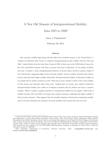
the fourth section, I present my estimates of intergenerational mobility in the early twentieth century forincome, education, and occupation, and compare these results to estimates for the modern period. I alsoconsider heterogeneity in the mobility parameters across my sample as well as geographic mobility. Sectionfive concludes the paper.2DataI draw my primary data for measuring intergenerational mobility in the United States early in the twentiethcentury from the 1915 Iowa State Census and the 1940 US Federal Census. The 1915 Iowa Census was acomplete survey of all 2.3 million Iowa residents in 1914. It was the first American census of any kind toinclude data on both annual income and years of education in addition to more traditional census measures,and it also includes respondent name, age, place of residence, birthplace, marital status, race, and occupation.I use the Iowa State Census sample digitised by Claudia Goldin and Lawrence Katz for their work on thehistorical returns to education (Goldin and Katz 2000, 2008). The Goldin-Katz sample includes 26,768 urbanresidents (5.5% of the total urban population of Iowa in 1915) and 33,305 rural residents (1.8% of the totalrural population). Figure 1 presents a map of the counties and cities included in the Goldin-Katz sample.The three large Iowa cities sampled are Des Moines, Davenport, and Dubuque.3 In 1915, the populationof Des Moines was approximately 97,000 people, making it the 64th largest city in the country. Davenportand Dubuque were smaller, with approximately 46,000 and 39,000 people, respectively. The rural countiesin the sample were selected by Goldin and Katz on the basis of both image and archive quality, as well asto provide a diverse geographic sample within the state, as shown in Figure 1.4To construct my sample for census matching, I limit the Goldin-Katz sample to families with boys agedbetween 3 and 17 in 1915. These sons will be between 28 and 42 when I observe them again in 1940, whichshould reduce measurement issues due to life cycle variability in annual income. I restrict my analysis tosons in 1915, because name changes make it impossible to locate most daughters in the 1940 Census. Thisleaves me with a sample of 7,580 boys, 6,071 of whom have fathers in their households and the requisite dataon both the father’s education and income. Each of those 7,580 observations is a son in 1915 Iowa.To locate these sons in 1940, I utilise the 100% 1940 census sample deposited by Ancestry.com withthe NBER. I collect the set of possible matches, using the son’s first and last name, middle initial (whenavailable), state of birth, and year of birth. Then, I train a record linking algorithm and use the scoresgenerated by that algorithm to identify the correct matches for each son from 1915 in the 1940 data.5 Once3 The census manuscripts for Sioux City, one of the other large cities in Iowa, was unreadable and not collected by Goldinand Katz (Goldin and Katz 2000).4 For more details on the construction of the Goldin-Katz sample, see Goldin and Katz (2000).5 I generate the training data used to train the algorithm by manually comparing a subset of sons from 1915 to the set4
LyonMitchellClayDubuqueBuchanan MarshallCarrollDes Moines JohnsonDavenport AdairMontgomeryFigure Wayne1: Map of Iowa 1915 Cities and County Samplethe matched sons are identified, I record the pertinent data from the 1940 records. The 1940 Census was thefirst federal census to collect data on incomes, weeks of work, and years of education of the entire population.6Because it is a national sample, I do not have to worry about losing many sons to out-migration, which mightotherwise bias my estimates.My match rate is roughly 59%, which is in line with the rates of previous literature linking betweencensuses.7 Table 2 shows my match rates for the rural and urban samples; match rates are comparablebetween the two samples. My sample size of 4,478 father-son pairs is also comparable to many otherprojects measuring intergenerational mobility, both historically (Long and Ferrie 2013) and recently (Leeof possible links in 1940 and determining which records are in fact matches for the same person. The match algorithm isused to reduce between-researcher variability in match quality, to speed up the matching process, and ensure data replication.The matching algorithm uses Jaro-Winkler string distances in first and last names, exact matches on state of birth, absolutedifference in year of birth, Soundex matches for first and last names, middle initial matches, matching first and last letters offirst and last names, and other record-based variables to predict whether a record is a true or false match. Based on crossvalidated out of sample predictions within my training data, the match algorithm has a true positive rate of nearly 90% and apositive prediction rate of 86%. For a detailed description of the matching algorithm, see a technical write up on my lications/automated-census-record-linking.6 Past federal censuses record contemporary school enrollment for each person (child), but not years of schooling completed for adults no longer in school. Earnings data was collected in 1940 only for wage and salary workers. The datacollected is the “total amount of money wages or salary” but enumerators were instructed: “Do not include the earning of businessmen, farmers, or professional persons derived from business profits, sale of corps, or fees.” For more, #584. The importance of this missing data will vary with the fraction of farmers and other business owners in my sample. It does not, however, affect farm labourers, whose earnings are reported the sameas other occupations. Of my matched sample, 13.7% of the sons in 1940 are farm owners or operators without income. Initially,I drop these observations with missing earnings data in analyses on income data. However, in Appendix 5, I impute earningsfor farmers using the 1950 census, which did collect data on capital income and non-wage and salary earnings. Using theseimputed earnings, I estimate even higher levels of mobility than in my main results.7 Parman (2011) reports match rates of just below 50%. Guest et al. (1989) match at 39.4%.5
and Solon 2009).Table 2: Sample Match ny project linking historical data is subject to possible bias due to the difficulty of making matchesbetween datasets. I present an analysis of potential bias in the matching below, which suggests that thefinal sample does not suffer any crucial construction defects. Simple transcription errors are the most likelyobstacle to linking between a son observed as a child in 1915 and as an adult in 1940. To test this, I calculatea number of string- and character-based statistics using the first and last names of the sons in my sample.First, I determine the name commonness of both the first and last name, relative to all names in thepooled IPUMS sample of the 1910 and 1920 censuses.8 A more common name is less likely to have aunique match in the 1940 Census, even after limiting the possible targets by state of birth and year ofbirth. Second, I calculate the length of each son’s first and last name. Longer names are more likely to beincorrectly transcribed, but they are also more likely to be distinctive.Third, I attempt to predict typographical errors using character similarity scores. Cognitive scientistsand typographers have studied how likely certain letters are to be mistaken for one another or how similartwo letters are visually. For example, readers are much more likely to mix up lower case p and q than theywould be p for k. Further, some letters are secularly more likely to be mis-transcribed than others: s is quitevisually unique while l and n are both visually similar to other letters.9 A name with a number of l’s or n’sin it is more likely to be mis-transcribed and thus not matched when I search in the 1940 Census.10 I use amatrix of letter visual similarity from Simpson et al. (2013) to compute, for first and last names, a similarityscore.118 The commonness statistic is measured as the share of 100 people in the pooled 1910 and 1920 sample with the same first(last) name. It ranges from 0.00118 (or roughly 1 person in 100,000 with the same name—these names are unique in my sample)to 1.72 for first names (John) or 1.02 for last names (Miller). Abramitzky et al. (2012) use relative commonness as a predictorof census match success as well.9 l is likely to be confused with f and i for example, while n is similar to both h and m.10 Recall matches are made using census indices transcribed by Ancestry.com and deposited with the NBER.11 Specifically, Simpson et al. (2013) conduct surveys of college students and other native and non-native English readers toassess the similarity of letters on a 7 point scale, where 7 indicates exactly the same and 1 extremely different. For example, iand l have a similarity score of 6.13, while w and t have a similarity score of exactly 1. I take the highest (non-self) similarityscore for each letter as a measure of a letter’s likelihood of being mis-transcribed. Figure A.1 in the appendix graphs thesescores for each letter. Then, I calculate the average of these scores for all letters in a given string (name). The scores fromSimpson et al are based on both lower case and upper case letters in block type. As many of the Census files are in script, avisual similarity matrix for cursive letters would be ideal, but such a measure does not exist in the typography literature. Asa robustness check, I also use a letter matrix of confusion probability from McGraw et al. (1994) and find a high correlationbetween each letter’s similarity score.6
Table 3: Probability of Matching a Record from Iowa 1915 to the Federal Census 1940(1)(2)(3)(4) (5)Name commonness, first name0.041(0.017)0.056 (0.020)Name commonness, last name 0.122 (0.039) 0.121 (0.039)0.013 (0.004)String length, first name0.020 (0.004) 0.002(0.004)String length, last name 0.002(0.004)Normalized letter similarity score, first name0.019 (0.007)0.024 (0.007)Normalized letter similarity score, last name0.006(0.007)0.005(0.007)Normalized scrabble score, first name 0.001(0.006) 0.002(0.007)Normalized scrabble score, last .007ObservationsClustersAdjusted R2758047310.002758047310.002758047310.001Linear probability model with an indicator variable for a successful match as the outcome. Standard errors areclustered by family. Results are consistent using a probit or logit model as well. Name commonness is measuredas the share of 100 men in the 1910 and 1920 IPUMS sample with the same first or last name. Name lengthis the number of characters in the first or last name. Name similarity scores are based on character typologysimilarity from Simpson et al. (2013).Sources: 1915 Iowa State Census Sample; 1940 Federal CensusFinally, I calculate a name’s Scrabble score as an alternative measure of both name commonness andname simplicity.12 Names with low Scrabble scores are likely to be made up of relatively common charactersand are less likely to be changed or Americanised over time (Biavaschi et al. 2013). I use standardised zscores for both the visual similarity scores and the Scrabble scores; the z-scores are based on the distributionof visual similarity scores and Scrabble scores within the pooled sample of my Iowa sons and the 1910 and1920 censuses.Table 3 presents the results from a series of linear probability models, predicting whether or not a sonin 1915 is uniquely matched ahead to the 1940 Federal Census. Sons with more common last names areless likely to be matched, while first name commonness has a smaller, positive effect. Sons with longer firstnames or first names with higher similarity scores are more likely to be found, but both of these effects arequite small.13 I include controls for all of these name string properties in all subsequent analysis.12 Biavaschi et al. (2013) introduce the use of Scrabble scores into the economic literature. They use this measure to predictname changes by immigrants to the United States during the early 20th century. Scrabble point values were based, originally,on the frequency of letters on US newspaper front pages.13 With controls for commonness and length, the Scrabble scores do not seem to relate to match rates.7
Table 4: Effects of Family Covariates on the Probability of Matching Records from 1915 to 1940Predicted Match Rate with X atXβSE25th Percentile75th PercentileFather Log EarningsFather EducationMother EducationUrban in 1915Son Born in IAFather Foreign .357.161.054.8This table presents the coefficients from a series of linear probability regressions with X as the primary independent variable, controlling for first and last name commonness, length, letter similarity, and Scrabble score. As inTable 3, there are 7580 observations and 4731 clusters, clustering standard errors by family.Sources: 1915 Iowa State Census Sample; 1940 Federal CensusMore serious issues could be generated by differential matching rates according to father, son, or familycharacteristics in 1915. In Table 4, I present the estimated effects of a set of variables observed for fathersand sons in 1915 on the probability of positively locating the son in the 1940 Census.14 Each row in the tableis a separate linear probability regression, reporting the coefficient of the listed X variable while controllingfor first and last name commonness, length, letter similarity, and Scrabble score. I am slightly more likely tomatch sons who had higher income or more educated fathers (or mothers) in 1915, but these effects are botheconomically and statistically insignificant. For example, the probability of matching a son with a father atthe 25th percentile of income is only 1 percentage points lower than matching a son with a father at the75th percentile of income. Similarly small effects of both father’s and mother’s education can be seen aswell. Confirming the results presented in Table 2, I am also less likely to match sons in the urban sample. Iam also more likely to link sons born in Iowa, even after conditioning on name string characteristics.15 Allanalysis undertaken in this paper will include controls for son’s place of birth, place of residence in 1915 and,where appropriate, father’s place of birth.The first two columns of Table 5 present summary statistics for the fathers of children between 3 and 17in the Goldin-Katz Iowa State Census sample. Observation counts are smaller than my full sample becausefathers of multiple children or sons are not double counted. The fathers in the sample are restricted tofathers of sons between 3 and 17; fathers found are the father for whom sons were located in the 1940 Censusthrough Ancestry.com. Average yearly earnings for the fathers are approximately 1000 in 1915 dollars. Theaverage father had a half year more than a common school education (eight years) and was approximately42 years old in 1915. Of the fathers in my sample, those fathers for whom I matched a son into the 194014 Results in this matching exercise are robust to alternative regression models, including logit and probit models. I use asimple linear probability model for ease of interpretation.15 86% of the sons in my sample were born in Iowa so there is no difference between the 25th to 75th percentile for thatcovariate.8
Table 5: Summary Statistics: Fathers in 1915 and Sons in 1915 and 1940FathersSonsFathers in SampleFound FathersSons in SampleSons FoundYearly Earnings1005.6(591.5)1007.1(587.6)1358.1(931.2)Log Yearly Earnings6.743(0.604)6.747(0.597)6.955(0.802)Log Weekly Earnings2.858(0.566)2.859(0.563)3.183(0.708)Years of Education8.491(2.837)8.507(2.803)10.61(3.092)Age 353)Born in 7)Urban 500)Observations3713220475802940All summary statistics are based on those fathers and sons with complete data for all listed variables. This restriction reduces the number of observations from the count of all sons found, as presented in Table 2. The samplefathers include only men with sons between the ages of 3 and 17 in 1915. The found fathers are only those menwith sons matched into the 1940 census. All sons includes any boys aged 3 to 17 in the Iowa sample in 1915; thefound sons are only those boys linked from 1915 to 1940. For fathers, earnings, education, age, and urban statusare measured in the 1915 Iowa State Census. For sons, earnings and education are measured in the 1940 FederalCensus, while age and urban status are measured in the 1915 Iowa State Census.Sources: 1915 Iowa State Census Sample; 1940 Federal CensusCensus earned very slightly more, though not significantly so, measured either in levels, logs, and weeklyearnings.The final two columns of Table 5 present summary statistics for the Iowa sons in my sample. Onlysummary data for sons with complete information in the 1940 Federal Census is reported in the table whichlowers the number of observations in the final column to 3,284. The located sons earned nearly 1400 in 1940,which is lower in real terms than the average earnings for their fathers in 1915, likely due to the lingeringeffects of the Great Depression.16 Also notable in the summary statistics is the fact that the sons had onaverage two more years of schooling than their fathers. This is a striking example of the effect of the highschool movement and the expansion of public education in Iowa, previously documented by Goldin and Katz(2008), Parman (2011), and others.How does my sample compare to the rest of the US in 1915 or in 1940? In Table 6, I compare the sonsin my sample to the national population in 1940, focusing on men aged 28 to 42. The second column is the16 Imeasure all dollar amounts in this paper in nominal terms. Because I use logged earnings in my regressions and income forall sons is measured in 1940 and for all fathers in 1915, any nominal to real conversions drop out into the unreported constantterm.9
Table 6: Summary Statistics: Sons in 1940Iowa Linked Sample1940 IPUMS SampleSons FoundUnweightedWeighted by State of BirthYearly Earnings1358.1(931.2)1237.2(889.4)1256.4(898.0)Log Yearly Earnings6.955(0.802)6.819(0.887)6.851(0.863)Log Weekly Earnings3.183(0.708)3.102(0.758)3.100(0.757)Years of Education10.61(3.092)9.151(3.482)10.29(2.980)Age .804(0.397)0.804(0.397)0.815(0.389)Born in Iowa0.869(0.337)0.0190(0.136)0.869(0.337)Share tions294011230999105All variables measured in 1940. After weighing the 1940 1% IPUMS sample of the census for state of birth, thematched sample of sons is comparable to the 1940 population of men between 28 and 42.Sources: 1940 Federal CensusIPUMS 1% sample of the 1940 census; the third column reweights the 1% sample by state of birth to matchthe states of birth in my Iowa sons sample. I find that my sample has slightly higher income than eitherthe general population or the reweighted sample. After reweighting, however, my sample is representativein terms of education, age, marital status, and race.1733.1Past Estimates of Intergenerational MobilityIntergenerational Income MobilityThe most frequent measure of intergenerational economic mobility used in the literature is the intergenerational elasticity of income (IGE), estimated by regressing the son’s log income against his father’s log income.Corak (2006), Solon (1999), and Black and Devereux (2011) present thorough reviews of the modern IGEliterature.18 These reviews all indicate a lack of historical data on intergenerational mobility: Corak (2006)documents 41 studies of the US IGE, none of which presents data before 1980. One aim of my project is to17 In a later analysis of geographic mobility, I show in Table 12 that my sample’s state of residence distribution in 1940 isroughly similar to the geographic distribution of all men born in Iowa between 1898 and 1912.18 The estimated elasticity of income between one generation and the next is commonly referred to as an IGE and I will usethat abbreviation here.10
establish a correct measure of
A New Old Measure of Intergenerational Mobility: Iowa 1915 to 1940 James J. Feigenbaumy February 20, 2015 . mobility between 1915 and 1940 to be larger than modern estimates, con rming the higher mobility I . making it the 64th largest city in the country. Davenport and Dubuque were smaller, with approximately 46,000 and 39,000 people .