Transcription
3THE LEAST-MEAN-SQUARE (LMS)ALGORITHM3.1INTRODUCTIONThe least-mean-square (LMS) is a search algorithm in which a simplification of the gradient vectorcomputation is made possible by appropriately modifying the objective function [1]-[2]. The LMSalgorithm, as well as others related to it, is widely used in various applications of adaptive filteringdue to its computational simplicity [3]-[7]. The convergence characteristics of the LMS algorithmare examined in order to establish a range for the convergence factor that will guarantee stability.The convergence speed of the LMS is shown to be dependent on the eigenvalue spread of theinput signal correlation matrix [2]-[6]. In this chapter, several properties of the LMS algorithmare discussed including the misadjustment in stationary and nonstationary environments [2]-[9] andtracking performance [10]-[12]. The analysis results are verified by a large number of simulationexamples. Appendix B, section B.1, complements this chapter by analyzing the finite-wordlengtheffects in LMS algorithms.The LMS algorithm is by far the most widely used algorithm in adaptive filtering for several reasons.The main features that attracted the use of the LMS algorithm are low computational complexity,proof of convergence in stationary environment, unbiased convergence in the mean to the Wienersolution, and stable behavior when implemented with finite-precision arithmetic. The convergenceanalysis of the LMS presented here utilizes the independence assumption.3.2THE LMS ALGORITHMIn Chapter 2 we derived the optimal solution for the parameters of the adaptive filter implementedthrough a linear combiner, which corresponds to the case of multiple input signals. This solution leadsto the minimum mean-square error in estimating the reference signal d(k). The optimal (Wiener)solution is given bywo R 1 p(3.1)where R E[x(k)xT (k)] and p E[d(k)x(k)], assuming that d(k) and x(k) are jointly wide-sensestationary.P.S.R. Diniz, Adaptive Filtering, DOI: 10.1007/978-0-387-68606-6 3, Springer Science Business Media, LLC 2008
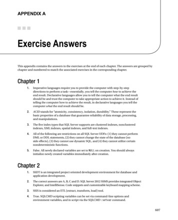
78Chapter 3 The Least-Mean-Square (LMS) AlgorithmIf good estimates of matrix R, denoted by R̂(k), and of vector p, denoted by p̂(k), are available,a steepest-descent-based algorithm can be used to search the Wiener solution of equation (3.1) asfollows:w(k 1) w(k) μĝw (k) w(k) 2μ(p̂(k) R̂(k)w(k))(3.2)for k 0, 1, 2, . . ., where ĝw (k) represents an estimate of the gradient vector of the objectivefunction with respect to the filter coefficients.One possible solution is to estimate the gradient vector by employing instantaneous estimates for Rand p as follows:R̂(k) x(k)xT (k)p̂(k) d(k)x(k)(3.3)The resulting gradient estimate is given byĝw (k) 2d(k)x(k) 2x(k)xT (k)w(k) 2x(k)( d(k) xT (k)w(k)) 2e(k)x(k)(3.4)Note that if the objective function is replaced by the instantaneous square error e2 (k), instead of theMSE, the above gradient estimate represents the true gradient vector since T e(k) e(k) e(k) e2 (k) 2e(k)2e(k). . . 2e(k) w w0 (k) w1 (k) wN (k) 2e(k)x(k) ĝw (k)(3.5)The resulting gradient-based algorithm is known1 as the least-mean-square (LMS) algorithm, whoseupdating equation isw(k 1) w(k) 2μe(k)x(k)(3.6)where the convergence factor μ should be chosen in a range to guarantee convergence.Fig. 3.1 depicts the realization of the LMS algorithm for a delay line input x(k). Typically, oneiteration of the LMS requires N 2 multiplications for the filter coefficient updating and N 1multiplications for the error generation. The detailed description of the LMS algorithm is shown inthe table denoted as Algorithm 3.1.It should be noted that the initialization is not necessarily performed as described in Algorithm 3.1,where the coefficients of the adaptive filter were initialized with zeros. For example, if a roughidea of the optimal coefficient value is known, these values could be used to form w(0) leading to areduction in the number of iterations required to reach the neighborhood of wo .1 Becauseit minimizes the mean of the squared error.
3.3 Some Properties of the LMS Algorithm79 z -1w0 (k) z -1w1 (k)x(k)z -1d(k)z -1 z -1 z -1y(k)- e(k)wN (k)2μFigure 3.13.3LMS adaptive FIR filter.SOME PROPERTIES OF THE LMS ALGORITHMIn this section, the main properties related to the convergence behavior of the LMS algorithm in astationary environment are described. The information contained here is essential to understand theinfluence of the convergence factor μ in various convergence aspects of the LMS algorithm.3.3.1 Gradient BehaviorAs shown in Chapter 2, see equation (2.91), the ideal gradient direction required to perform a searchon the MSE surface for the optimum coefficient vector solution is gw (k) 2{E x(k)xT (k) w(k) E [d(k)x(k)]} 2[Rw(k) p](3.7)
80Chapter 3 The Least-Mean-Square (LMS) AlgorithmAlgorithm 3.1LMS AlgorithmInitializationx(0) w(0) [0 0 . . . 0]TDo for k 0e(k) d(k) xT (k)w(k)w(k 1) w(k) 2μe(k)x(k)In the LMS algorithm, instantaneous estimates of R and p are used to determine the search direction,i.e., ĝw (k) 2 x(k)xT (k)w(k) d(k)x(k)(3.8)As can be expected, the direction determined by equation (3.8) is quite different from that of equation (3.7). Therefore, by using the more computationally attractive gradient direction of the LMSalgorithm, the convergence behavior is not the same as that of the steepest-descent algorithm.On average, it can be said that the LMS gradient direction has the tendency to approach the idealgradient direction since for a fixed coefficient vector w E[ĝw (k)] 2{E x(k)xT (k) w E [d(k)x(k)]} gw(3.9)hence, vector ĝw (k) can be interpreted as an unbiased instantaneous estimate of gw . In an ergodicenvironment, if, for a fixed w vector, ĝw (k) is calculated for a large number of inputs and referencesignals, the average direction tends to gw , i.e.,M1 ĝw (k i) gwM Mi 1lim(3.10)3.3.2 Convergence Behavior of the Coefficient VectorAssume that an unknown FIR filter with coefficient vector given by wo is being identified by anadaptive FIR filter of the same order, employing the LMS algorithm. Measurement white noise n(k)with zero mean and variance σn2 is added to the output of the unknown system.
3.3 Some Properties of the LMS Algorithm81The error in the adaptive-filter coefficients as related to the ideal coefficient vector wo , in eachiteration, is described by the N 1-length vectorΔw(k) w(k) wo(3.11)With this definition, the LMS algorithm can alternatively be described byΔw(k 1) Δw(k) 2μe(k)x(k) Δw(k) 2μx(k) xT (k)wo n(k) xT (k)w(k) Δw(k) 2μx(k) eo (k) xT (k)Δw(k) I 2μx(k)xT (k) Δw(k) 2μeo (k)x(k)(3.12)where eo (k) is the optimum output error given byeo (k) d(k) wTo x(k) wTo x(k) n(k) wTo x(k)(3.13) n(k)The expected error in the coefficient vector is then given byE[Δw(k 1)] E{[I 2μx(k)xT (k)]Δw(k)} 2μE[eo (k)x(k)](3.14)If it is assumed that the elements of x(k) are statistically independent of the elements of Δw(k) andeo (k), equation (3.14) can be simplified as follows:E[Δw(k 1)] {I 2μE[x(k)xT (k)]}E[Δw(k)] (I 2μR)E[Δw(k)](3.15)The first assumption is justified if we assume that the deviation in the parameters is dependent onprevious input signal vectors only, whereas in the second assumption we also considered that theerror signal at the optimal solution is orthogonal to the elements of the input signal vector. The aboveexpression leads toE[Δw(k 1)] (I 2μR)k 1 E[Δw(0)](3.16)Equation (3.15) premultiplied by QT , where Q is the unitary matrix that diagonalizes R through asimilarity transformation, yields E QT Δw(k 1) (I 2μQT RQ)E QT Δw(k) E [Δw (k 1)] (I 2μΛ)E [Δw (k)] 1 2μλ00 01 2μλ1 . .00···.0.1 2μλN E [Δw (k)] (3.17)
82Chapter 3 The Least-Mean-Square (LMS) Algorithmwhere Δw (k 1) QT Δw(k 1) is the rotated-coefficient error vector. The applied rotationyielded an equation where the driving matrix is diagonal, making it easier to analyze the equation’sdynamic behavior. Alternatively, the above relation can be expressed asE [Δw (k 1)] (I 2μΛ)k 1 E [Δw (0)] (1 2μλ0 )k 10 0(1 2μλ1 )k 1 . .00···.0.(1 2μλN )k 1 E [Δw (0)] (3.18)This equation shows that in order to guarantee convergence of the coefficients in the mean, theconvergence factor of the LMS algorithm must be chosen in the range0 μ 1λmax(3.19)where λmax is the largest eigenvalue of R. Values of μ in this range guarantees that all elements ofthe diagonal matrix in equation (3.18) tend to zero as k , since 1 (1 2μλi ) 1, fori 0, 1, . . . , N . As a result E[Δw (k 1)] tends to zero for large k.The choice of μ as above explained ensures that the mean value of the coefficient vector approachesthe optimum coefficient vector wo . It should be mentioned that if the matrix R has a large eigenvaluespread, it is advisable to choose a value for μ much smaller than the upper bound. As a result,the convergence speed of the coefficients will be primarily dependent on the value of the smallesteigenvalue, responsible for the slowest mode in equation (3.18).The key assumption for the above analysis is the so-called independence theory [4], which considersall vectors x(i), for i 0, 1, . . . , k, statistically independent. This assumption allowed us to consider Δw(k) independent of x(k)xT (k) in equation (3.14). Such an assumption, despite not beingrigorously valid especially when x(k) consists of the elements of a delay line, leads to theoreticalresults that are in good agreement with the experimental results.3.3.3 Coefficient-Error-Vector Covariance MatrixIn this subsection, we derive the expressions for the second-order statistics of the errors in theadaptive-filter coefficients. Since for large k the mean value of Δw(k) is zero, the covariance of thecoefficient-error vector is defined ascov[Δw(k)] E[Δw(k)ΔwT (k)] E{[w(k) wo ][w(k) wo ]T }(3.20)
3.3 Some Properties of the LMS Algorithm83By replacing equation (3.12) in (3.20) it follows that T cov[Δw(k 1)] E{ I 2μx(k)xT (k) Δw(k)ΔwT (k) I 2μx(k)xT (k) [I 2μx(k)xT (k)]Δw(k)2μeo (k)xT (k) 2μeo (k)x(k)ΔwT (k)[I 2μx(k)xT (k)]T 4μ2 e2o (k)x(k)xT (k)}(3.21)By considering eo (k) independent of Δw(k) and orthogonal to x(k), the second and third terms onthe right-hand side of the above equation can be eliminated. The details of this simplification can becarried out by describing each element of the eliminated matrices explicitly. In this case,cov[Δw(k 1)] cov[Δw(k)] E[ 2μx(k)xT (k)Δw(k)ΔwT (k) 2μΔw(k)ΔwT (k)x(k)xT (k) 4μ2 x(k)xT (k)Δw(k)ΔwT (k)x(k)xT (k) 4μ2 e2o (k)x(k)xT (k)](3.22)In addition, assuming that Δw(k) and x(k) are independent, equation (3.22) can be rewritten ascov[Δw(k 1)] cov[Δw(k)] 2μE[x(k)xT (k)]E[Δw(k)ΔwT (k)] 2μE[Δw(k)ΔwT (k)]E[x(k)xT (k)] 4μ2 E x(k)xT (k)E[Δw(k)ΔwT (k)]x(k)xT (k) 4μ2 E[e2o (k)]E[x(k)xT (k)] cov[Δw(k)] 2μR cov[Δw(k)] 2μ cov[Δw(k)]R 4μ2A 4μ2 σn2 R(3.23) The calculation of A E x(k)xT (k)E[Δw(k)ΔwT (k)]x(k)xT (k) involves fourth-order moments and the result can be obtained by expanding the matrix inside the operation E[·] as describedin [4] and [13] for jointly Gaussian input signal samples. The result isA 2R cov[Δw(k)] R R tr{R cov[Δw(k)]}(3.24)where tr[·] denotes trace of [·]. Equation (3.23) is needed to calculate the excess mean-square errorcaused by the noisy estimate of the gradient employed by the LMS algorithm. As can be noted,cov[Δw(k 1)] does not tend to 0 as k , due to the last term in equation (3.23) that providesan excitation in the dynamic matrix equation.A more useful form for equation (3.23) can be obtained by premultiplying and postmultiplying it byQT and Q respectively, yieldingQT cov[Δw(k 1)]Q QT cov[Δw(k)] Q 2μQT RQQT cov[Δw(k)]Q 2μQT cov[Δw(k)]QQT RQ 8μ2 QT RQQT cov[Δw(k)]QQT RQ 4μ2 QT RQQT tr{RQQT cov[Δw(k)]}Q 4μ2 σn2 QT RQ(3.25)
84Chapter 3 The Least-Mean-Square (LMS) Algorithmwhere we used the equality QT Q QQT I. Using the fact that QT tr[B]Q tr[QT BQ]I forany B,cov[Δw (k 1)] cov[Δw (k)] 2μΛ cov[Δw (k)] 2μ cov[Δw (k)]Λ 8μ2 Λ cov[Δw (k)]Λ 4μ2 Λ tr{Λ cov[Δw (k)]} 4μ2 σn2 Λ(3.26)where cov[Δw (k)] E[QT Δw(k)ΔwT (k)Q].As will be shown in subsection 3.3.6, only the diagonal elements of cov[Δw (k)] contribute to theexcess MSE in the LMS algorithm. By defining v (k) as a vector with elements consisting of thediagonal elements of cov[Δw (k)], and λ as a vector consisting of the eigenvalues of R, the followingrelation can be derived from the above equationsv (k 1) (I 4μΛ 8μ2 Λ2 4μ2 λλT )v (k) 4μ2 σn2 λ Bv (k) 4μ2 σn2 λ(3.27)where the elements of B are given by 1 4μλi 8μ2 λ2i 4μ2 λ2ibij 4μ2 λi λjfor i j(3.28)for i jThe value of the convergence factor μ must be chosen in a range that guarantees the convergenceof v (k). Since matrix B is symmetric, it has only real-valued eigenvalues. Also since all entries ofB are also non-negative, the maximum among the sum of elements in any row of B represents anupper bound to the maximum eigenvalue of B and to the absolute value of any other eigenvalue, seepages 53 and 63 of [14] or the Gershgorin theorem in [15]. As a consequence, a sufficient conditionto guaranteeconvergence is to force the sum of the elements in any row of B to be kept in the range N0 j 0 bij 1. SinceN bij 1 4μλi 8μ2 λ2i 4μ2 λiN j 0λj(3.29)j 0the critical values of μ are those for which the above equation approaches 1, as for any μ the expressionis always positive. This will occur only if the last three terms of equation (3.29) approach zero, that is 4μλi 8μ2 λ2i 4μ2 λiN λj 0j 0After simple manipulation the stability condition obtained is0 μ 111 N Ntr[R]2λmax j 0 λjj 0 λj(3.30)where the last and simpler expression is more widely used in practice because tr[R] is quite simpleto estimate since it is related with the Euclidean norm squared of the input signal vector, whereas an
3.3 Some Properties of the LMS Algorithm85estimate λmax is much more difficult to obtain. It will be shown in equation (3.45) that μ controlsthe speed of convergence of the MSE.The upper bound obtained for the value of μ is important from the practical point of view, because itgives us an indication of the maximum value of μ that could be used in order to achieve convergenceof the coefficients. However, the reader should be advised that the given upper bound is somewhatoptimistic due to the approximations and assumptions made. In most cases, the value of μ shouldnot be chosen close to the upper bound.3.3.4 Behavior of the Error SignalIn this subsection, the mean value of the output error in the adaptive filter is calculated, consideringthat the unknown system model has infinite impulse response and there is measurement noise. Theerror signal, when an additional measurement noise is accounted for, is given bye(k) d (k) wT (k)x(k) n(k)(3.31)where d (k) is the desired signal without measurement noise. For a given known input vector x(k),the expected value of the error signal isE[e(k)] E[d (k)] E[wT (k)x(k)] E[n(k)] E[d (k)] wTo x(k) E[n(k)](3.32)where wo is the optimal solution, i.e., the Wiener solution for the coefficient vector. Note thatthe input signal vector was assumed known in the above equation, in order to expose what can beexpected if the adaptive filter converges to the optimal solution. If d (k) was generated through aninfinite impulse response system, a residue error remains in the subtraction of the first two terms dueto undermodeling (adaptive FIR filter with insufficient number of coefficients), i.e., E[e(k)] Eh(i)x(k i) E[n(k)](3.33)i N 1where h(i), for i N 1, . . . , , are the coefficients of the process that generated the part of d (k)not identified by the adaptive filter. If the input signal and n(k) have zero mean, then E[e(k)] 0.3.3.5 Minimum Mean-Square ErrorIn this subsection, the minimum MSE is calculated for undermodeling situations and in the presenceof additional noise. Let’s assume again the undermodeling case where the adaptive filter has lesscoefficients than the unknown system in a system identification setup. In this case we can writed(k) hT x (k) n(k) Tx(k)T [wo h ] n(k)x (k)(3.34)
86Chapter 3 The Least-Mean-Square (LMS) Algorithmwhere wo is a vector containing the first N 1 coefficients of the unknown system impulse response,h contains the remaining elements of h. The output signal of an adaptive filter with N 1 coefficientsis given byy(k) wT (k)x(k)In this setup the MSE has the following expressionTξ E{d2 (k) 2wTo x(k)wT (k)x(k) 2h x (k)wT (k)x(k) 2[wT (k)x(k)]n(k) [wT (k)x(k)]2 } Tx(k)x(k)T2TT E d (k) 2[w (k) 0 ][wo h ]x (k)x (k) TT2 2[w (k)x(k)]n(k) [w (k)x(k)] woT2T E[d (k)] 2[w (k) 0 ]R wT (k)Rw(k)h whereR Ex(k)x (k) (3.35) T[x (k)xT (k)]and 0 is an infinite length vector whose elements are zeros. By calculating the derivative of ξwith respect to the coefficients of the adaptive filter, it follows that (see derivations around equations(2.91) and (2.148)) woŵo R 1 trunc {p }N 1 R 1 trunc R hN 1 R 1 trunc{R h}N 1(3.36)where trunc{a}N 1 represents a vector generated by retaining the first N 1 elements of a. Itshould be noticed that the results of equations (3.35) and (3.36) are algorithm independent.The minimum mean-square error can be obtained from equation (3.35), when assuming the inputsignal is a white noise uncorrelated with the additional noise signal, that isξmin E[e2 (k)]min h2 (i)E[x2 (k i)] E[n2 (k)]i N 1 h2 (i)σx2 σn2(3.37)i N 1This minimum error is achieved when it is assumed that the adaptive-filter multiplier coefficients arefrozen at their optimum values, refer to equation (2.148) for similar discussion. In case the adaptivefilter has sufficient order to model the process that generated d(k), the minimum MSE that can beachieved is equal to the variance of the additional noise, given by σn2 . The reader should note that theeffect of undermodeling discussed in this subsection generates an excess MSE with respect to σn2 .
3.3 Some Properties of the LMS Algorithm873.3.6 Excess Mean-Square Error and MisadjustmentThe result of the previous subsection assumes that the adaptive-filter coefficients converge to theiroptimal values, but in practice this is not so. Although the coefficient vector on average convergesto wo , the instantaneous deviation Δw(k) w(k) wo , caused by the noisy gradient estimates,generates an excess MSE. The excess MSE can be quantified as described in the present subsection.The output error at instant k is given bye(k) d(k) wTo x(k) ΔwT (k)x(k) eo (k) ΔwT (k)x(k)(3.38)thene2 (k) e2o (k) 2eo (k)ΔwT (k)x(k) ΔwT (k)x(k)xT (k)Δw(k)(3.39)The so-called independence theory assumes that the vectors x(k), for all k, are statistically independent, allowing a simple mathematical treatment for the LMS algorithm. As mentioned before, thisassumption is in general not true, especially in the case where x(k) consists of the elements of a delayline. However, even in this case the use of the independence assumption is justified by the agreementbetween the analytical and the experimental results. With the independence assumption, Δw(k) canbe considered independent of x(k), since only previous input vectors are involved in determiningΔw(k). By using the assumption and applying the expected value operator to equation (3.39), wehaveξ(k) E[e2 (k)] ξmin 2E[ΔwT (k)]E[eo (k)x(k)] E[ΔwT (k)x(k)xT (k)Δw(k)] ξmin 2E[ΔwT (k)]E[eo (k)x(k)] E{tr[ΔwT (k)x(k)xT (k)Δw(k)]} ξmin 2E[ΔwT (k)]E[eo (k)x(k)] E{tr[x(k)xT (k)Δw(k)ΔwT (k)]}(3.40)where in the fourth equality we used the property tr[A · B] tr[B · A]. The last term of the aboveequation can be rewritten as tr E[x(k)xT (k)]E[Δw(k)ΔwT (k)]Since R E[x(k)xT (k)] and by the orthogonality principle E[eo (k)x(k)] 0, the above equationcan be simplified as follows:ξ(k) ξmin E[ΔwT (k)RΔw(k)](3.41)The excess in the MSE is given by Δξ(k) ξ(k) ξmin E[ΔwT (k)RΔw(k)] E{tr[RΔw(k)ΔwT (k)]} tr{E[RΔw(k)ΔwT (k)]}(3.42)By using the fact that QQT I, the following relation results Δξ(k) tr E[QQT RQQT Δw(k)ΔwT (k)QQT ] tr{QΛ cov[Δw (k)]QT }(3.43)
88Chapter 3 The Least-Mean-Square (LMS) AlgorithmTherefore,Δξ(k) tr{Λ cov[Δw (k)]}(3.44)From equation (3.27), it is possible to show thatΔξ(k) N λi vi (k) λT v (k)(3.45)i 0Sincevi (k 1) (1 4μλi 8μ2 λ2i )vi (k) 4μ2 λiN λj vj (k) 4μ2 σn2 λi(3.46)j 0and vi (k 1) vi (k) for large k, we can apply a summation operation to the above equation inorder to obtain N NN μσn2 i 0 λi 2μ i 0 λ2i vi (k)λj vj (k) N1 μ i 0 λij 0 Nμσn2 i 0 λi N1 μ i 0 λi μσn2 tr[R]1 μtr[R](3.47) Nwhere the term 2μ i 0 λ2i vi (k) was considered very small as compared to the remaining terms ofthe numerator. This assumption is not easily justifiable, but is valid for small values of μ.The excess mean-square error can then be expressed asξexc lim Δξ(k) k μσn2 tr[R]1 μtr[R](3.48)This equation, for very small μ, can be approximated byξexc μσn2 tr[R] μ(N 1)σn2 σx2(3.49)where σx2 is the input signal variance and σn2 is the additional-noise variance.The misadjustment M , defined as the ratio between the ξexc and the minimum MSE, is a commonparameter used to compare different adaptive signal processing algorithms. For the LMS algorithm,the misadjustment is given byμtr[R] ξexc(3.50)M ξmin1 μtr[R]
3.3 Some Properties of the LMS Algorithm893.3.7 Transient BehaviorBefore the LMS algorithm reaches the steady-state behavior, a number of iterations are spent in thetransient part. During this time, the adaptive-filter coefficients and the output error change from theirinitial values to values close to that of the corresponding optimal solution.In the case of the adaptive-filter coefficients, the convergence in the mean will follow (N 1)geometric decaying curves with ratios rwi (1 2μλi ). Each of these curves can be approximatedby an exponential envelope with time constant τwi as follows (see equation (3.18)) [2]: 1rwi e τwi 1 11 2 ···τwi2!τwi(3.51)where for each iteration, the decay in the exponential envelope is equal to the decay in the originalgeometric curve. In general, rwi is slightly smaller than one, especially for the slowly decreasingmodes corresponding to small λi and μ. Therefore,rwi (1 2μλi ) 1 thenτwi 1τwi(3.52)12μλifor i 0, 1, . . . , N . Note that in order to guarantee convergence of the tap coefficients in the mean,μ must be chosen in the range 0 μ 1/λmax (see equation (3.19)).According to equation (3.30), for the convergence of the MSE the range of values for μ is 0 μ 1/tr[R], and the corresponding time constant can be calculated from matrix B in equation (3.27), byconsidering the terms in μ2 small as compared to the remaining terms in matrix B. In this case, thegeometric decaying curves have ratios given by rei (1 4μλi ) that can be fitted to exponentialenvelopes with time constants given byτei 14μλi(3.53)for i 0, 1, . . . , N . In the convergence of both the error and the coefficients, the time required forthe convergence depends on the ratio of eigenvalues of the input signal correlation matrix.Returning to the tap coefficients case, if μ is chosen to be approximately 1/λmax the correspondingtime constant for the coefficients is given byτwi λmaxλmax 2λi2λmin(3.54)Since the mode with the highest time constant takes longer to reach convergence, the rate of convergence is determined by the slowest mode given by τwmax λmax /(2λmin ). Suppose the convergenceis considered achieved when the slowest mode provides an attenuation of 100, i.e., ke τwmax 0.01
90Chapter 3 The Least-Mean-Square (LMS) Algorithmthis requires the following number of iterations in order to reach convergence:k 4.6λmax2λminThe above situation is quite optimistic because μ was chosen to be high. As mentioned before, inpractice we should choose the value of μ much smaller than the upper bound. For an eigenvalue spreadapproximating one, according to equation (3.30) let’s choose μ smaller than 1/[(N 3)λmax ].2 Inthis case, the LMS algorithm will require at leastk 4.6(N 3)λmax 2.3(N 3)2λminiterations to achieve convergence in the coefficients.The analytical results presented in this section are valid for stationary environments. The LMSalgorithm can also operate in the case of nonstationary environments, as shown in the followingsection.3.4LMS ALGORITHM BEHAVIOR IN NONSTATIONARYENVIRONMENTSIn practical situations, the environment in which the adaptive filter is embedded may be nonstationary.In these cases, the input signal autocorrelation matrix and/or the cross-correlation vector, denotedrespectively by R(k) and p(k), are/is varying with time. Therefore, the optimal solution for thecoefficient vector is also a time-varying vector given by wo (k).Since the optimal coefficient vector is not fixed, it is important to analyze if the LMS algorithmwill be able to track changes in wo (k). It is also of interest to learn how the tracking error in thecoefficients given by E[w(k)] wo (k) will affect the output MSE. It will be shown later that theexcess MSE caused by lag in the tracking of wo (k) can be separated from the excess MSE causedby the measurement noise, and therefore, without loss of generality, in the following analysis theadditional noise will be considered zero.The coefficient-vector updating in the LMS algorithm can be written in the following formw(k 1) w(k) 2μx(k)e(k) w(k) 2μx(k)[d(k) xT (k)w(k)](3.55)Sinced(k) xT (k)wo (k)(3.56)the coefficient updating can be expressed as follows:w(k 1) w(k) 2μx(k)[xT (k)wo (k) xT (k)w(k)]2 Thischoice also guarantees the convergence of the MSE.(3.57)
3.4 LMS Algorithm Behavior in Nonstationary Environments91Now assume that an ensemble of a nonstationary adaptive identification process has been built, wherethe input signal in each experiment is taken from the same stochastic process. The input signal isconsidered stationary. This assumption results in a fixed R matrix, and the nonstationarity is caused bythe desired signal that is generated by applying the input signal to a time-varying system. With theseassumptions, by using the expected value operation to the ensemble, with the coefficient updatingin each experiment given by equation (3.57), and additionally assuming that w(k) is independent ofx(k) yieldsE[w(k 1)] E[w(k)] 2μE[x(k)xT (k)]wo (k) 2μE[x(k)xT (k)]E[w(k)] E[w(k)] 2μR{wo (k) E[w(k)]}(3.58)If the lag in the coefficient vector is defined bylw (k) E[w(k)] wo (k)(3.59)lw (k 1) (I 2μR)lw (k) wo (k 1) wo (k)(3.60)equation (3.58) can be rewritten asIn order to simplify our analysis, we can premultiply the above equation by QT , resulting in adecoupled set of equations given byl w (k 1) (I 2μΛ)l w (k) w o (k 1) w o (k)(3.61)where the vectors with superscript are the original vectors projected onto the transformed space. Ascan be noted, each element of the lag-error vector is determined by the following relation (k 1) woi(k)li (k 1) (1 2μλi )li (k) woi(3.62)where li (k) is the ith element of l w (k). By properly interpreting the above equation, we can say thatthe lag is generated by applying the transformed instantaneous optimal coefficient to a first-order discrete-time lag filter denoted as Li (z), i.e.,L i (z) z 1 Woi(z) Li (z)Woi(z)z 1 2μλi(3.63)The discrete-time filter transient response converges with a time constant of the exponential envelopegiven by1(3.64)τi 2μλiwhich is of course different for each individual tap. Therefore, the tracking ability of the coefficientsin the LMS algorithm is dependent on the eigenvalues of the input signal correlation matrix.The lag in the adaptive-filter coefficients leads to an excess mean-square error. In order to calculatethe excess MSE, suppose that each element of the optimal coefficient vector is modeled as a first-orderMarkov process. This nonstationary situation can be considered somewhat simplified as comparedwith some real practical situations. However, it allows a manageable mathematical analysis while
92Chapter 3 The Least-Mean-Square (LMS) Algorithmretaining the essence of handling the more complicated cases. The first-order Markov process isdescribed bywo (k) λw wo (k 1) nw (k)(3.65)2where nw (k) is a vector whose elements are zero-mean white noise processes with variance σw, andλw 1. Note that (1 2μλi ) λw 1, for i 0, 1, . . . , N , since the optimal coefficients values11must vary slower than the adaptive-filter tracking speed, i.e., 2μλ 1 λ. This model may notiwTrepresent an actual system when λw 1, since the E[wo (k)wo (k)] will have unbounded elementsif, for example, nw (k) is not exactly zero mean. A more realistic model would include a factorp(1 λw ) 2 , for p 1, multiplying nw (k) in order to guarantee that E[wo (k)wTo (k)] is bounded.In the following discussions, this case will not be considered since the corresponding results can beeasily derived (see problem 14).From equations (3.62) and (3.63), we can infer that the lag-error vector elements are generatedby applying a first-order discrete-time system to the elements of the unknown system coefficientvector, both in the transformed space. On the other hand, the coefficients of the unknown systemare generated by applying each element of the noise vector nw (k) to a first-order all-pole filter,with the pole placed at λw . For the unknown coefficient vector with the above model, the lagerror vector elements can be generated by applying each element of the transformed noise vectorn w (k) QT nw (k) to a discrete-time filter with transfer functionHi (z) (z 1)z(z 1 2μλi )(z λw )(3.66) This transfer func
The resulting gradient-based algorithm is known1 as the least-mean-square (LMS) algorithm, whose updating equation is w(k 1) w(k) 2μe(k)x(k) (3.6) where the convergence factor μshould be chosen in a range to guarantee convergence. Fig. 3.1 depicts the realization of the LMS algorithm for a delay line input x(k). Typically, one