Transcription
Introduction to Tensor CalculusKees Dullemond & Kasper Peetersc 1991-2010
This booklet contains an explanation about tensor calculus for students of physicsand engineering with a basic knowledge of linear algebra. The focus lies mainly onacquiring an understanding of the principles and ideas underlying the concept of‘tensor’. We have not pursued mathematical strictness and pureness, but insteademphasise practical use (for a more mathematically pure resumé, please see the bibliography). Although tensors are applied in a very broad range of physics and mathematics, this booklet focuses on the application in special and general relativity.We are indebted to all people who read earlier versions of this manuscript and gaveuseful comments, in particular G. Bäuerle (University of Amsterdam) and C. Dullemond Sr. (University of Nijmegen).The original version of this booklet, in Dutch, appeared on October 28th, 1991. Amajor update followed on September 26th, 1995. This version is a re-typeset Englishtranslation made in 2008/2010.Copyright c 1991-2010 Kees Dullemond & Kasper Peeters.
1The index notation2Bases, co- and contravariant vectors2.1 Intuitive approach . . . . . . . . . . . . . . . . . . . . . . . . . . . . .2.2 Mathematical approach . . . . . . . . . . . . . . . . . . . . . . . . . .99113Introduction to tensors3.1 The new inner product and the first tensor . . . . . . . . . . . . . . .3.2 Creating tensors from vectors . . . . . . . . . . . . . . . . . . . . . . .1515174Tensors, definitions and properties4.1 Definition of a tensor . . . . . .4.2 Symmetry and antisymmetry .4.3 Contraction of indices . . . . .4.4 Tensors as geometrical objects .4.5 Tensors as operators . . . . . .2121212222245The metric tensor and the new inner product5.1 The metric as a measuring rod . . . . . . . . . . . . . . . . . . . . . . .5.2 Properties of the metric tensor . . . . . . . . . . . . . . . . . . . . . . .5.3 Co versus contra . . . . . . . . . . . . . . . . . . . . . . . . . . . . . . .252526276Tensor calculus6.1 The ‘covariance’ of equations . . . . . . . . . . .6.2 Addition of tensors . . . . . . . . . . . . . . . . .6.3 Tensor products . . . . . . . . . . . . . . . . . . .6.4 First order derivatives: non-covariant version . .6.5 Rot, cross-products and the permutation symbol.292930313132Covariant derivatives7.1 Vectors in curved coordinates . . . . . . . . . . . . . . . . . . . . . . .7.2 The covariant derivative of a vector/tensor field . . . . . . . . . . . .35353675.A Tensors in special relativity39B Geometrical representation41C ExercisesC.1 Index notation . . . . .C.2 Co-vectors . . . . . . .C.3 Introduction to tensorsC.4 Tensoren, algemeen . .C.5 Metrische tensor . . . .C.6 Tensor calculus . . . .474749495051513
4
1The index notationBefore we start with the main topic of this booklet, tensors, we will first introduce anew notation for vectors and matrices, and their algebraic manipulations: the indexnotation. It will prove to be much more powerful than the standard vector notation. To clarify this we will translate all well-know vector and matrix manipulations(addition, multiplication and so on) to index notation.Let us take a manifold ( space) with dimension n. We will denote the components of a vector v with the numbers v1 , . . . , v n . If one modifies the vector basis, inwhich the components v1 , . . . , v n of vector v are expressed, then these componentswill change, too. Such a transformation can be written using a matrix A, of whichthe columns can be regarded as the old basis vectors e1 , . . . , en expressed in the newbasis e1 ′ , . . . , en ′ , ′ v1A11 · · · A1nv1 . . . (1.1) . . . v′n···An1AnnvnNote that the first index of A denotes the row and the second index the column. Inthe next chapter we will say more about the transformation of vectors.According to the rules of matrix multiplication the above equation means:v1′.v′n A11 · v1. An1 · v1 A12 · v2. ··· An2 · v2 ··· A1n · vn ,.(1.2)Ann · vn ,or equivalently,v1′ .v′n n A1ν vν ,ν 1.(1.3)n Anν vν ,ν 1or even shorter,v′µ n Aµν vνν 1( µ N 1 µ n) .(1.4)In this formula we have put the essence of matrix multiplication. The index ν is adummy index and µ is a running index. The names of these indices, in this case µ and5
CHAPTER 1. THE INDEX NOTATIONν, are chosen arbitrarily. The could equally well have been called α and β:nv′α Aαβ v β( α N 1 α n) .β 1(1.5)Usually the conditions for µ (in Eq. 1.4) or α (in Eq. 1.5) are not explicitly statedbecause they are obvious from the context.The following statements are therefore equivalent: v y v A yvµ yµ vα yα ,n vµ Aµν yνν 1n vν Aνµ yµ .(1.6)µ 1This index notation is also applicable to other manipulations, for instance the innerproduct. Take two vectors v and w , then we define the inner product asn v · w : v 1 w1 · · · v n w n vµ wµ .(1.7)µ 1(We will return extensively to the inner product. Here it is just as an example of thepower of the index notation). In addition to this type of manipulations, one can alsojust take the sum of matrices and of vectors:C A B z v w Cµν Aµν Bµν(1.8) Cµν Aµν Bµν(1.9) zα vα wαor their difference,C A B z v w zα vα wαExercises 1 to 6 of Section C.1.From the exercises it should have become clear that the summation symbols can always be put at the start of the formula and that their order is irrelevant. We cantherefore in principle omit these summation symbols, if we make clear in advanceover which indices we perform a summation, for instance by putting them after theformula,n Aµν vνν 1n Aµν vν{ν }(1.10)n β 1 γ 1Aαβ Bβγ Cγδ Aαβ Bβγ Cγδ{ β, γ}From the exercises one can already suspect that almost never is a summation performed over an index if that index only appears once in a product, almost always a summation is performed over an index that appears twice ina product, an index appears almost never more than twice in a product.6
CHAPTER 1. THE INDEX NOTATIONWhen one uses index notation in every day routine, then it will soon becomeirritating to denote explicitly over which indices the summation is performed. Fromexperience (see above three points) one knows over which indices the summationsare performed, so one will soon have the idea to introduce the convention that,unless explicitly stated otherwise: a summation is assumed over all indices that appear twice in a product, and no summation is assumed over indices that appear only once.From now on we will write all our formulae in index notation with this particularconvention, which is called the Einstein summation convection. For a more detailedlook at index notation with the summation convention we refer to [4]. We will thusfrom now on rewriten Aµν vνν 1nAµν vν , Aαβ Bβγ Cγδ .(1.11)n Aαβ Bβγ Cγδβ 1 γ 1 Exercises 7 to 10 of Section C.1.7
CHAPTER 1. THE INDEX NOTATION8
2Bases, co- and contravariant vectorsIn this chapter we introduce a new kind of vector (‘covector’), one that will be essential for the rest of this booklet. To get used to this new concept we will first showin an intuitive way how one can imagine this new kind of vector. After that we willfollow a more mathematical approach.2.1. Intuitive approachWe can map the space around us using a coordinate system. Let us assume thatwe use a linear coordinate system, so that we can use linear algebra to describeit. Physical objects (represented, for example, with an arrow-vector) can then bedescribed in terms of the basis-vectors belonging to the coordinate system (thereare some hidden difficulties here, but we will ignore these for the moment). Inthis section we will see what happens when we choose another set of basis vectors,i.e. what happens upon a basis transformation.In a description with coordinates we must be fully aware that the coordinates(i.e. the numbers) themselves have no meaning. Only with the corresponding basisvectors (which span up the coordinate system) do these numbers acquire meaning.It is important to realize that the object one describes is independent of the coordinate system (i.e. set of basis vectors) one chooses. Or in other words: an arrow doesnot change meaning when described an another coordinate system.Let us write down such a basis transformation, e1 ′ a11 e1 a12 e2 ,′ a21 e1 a22 e2 . e2(2.1)This could be regarded as a kind of multiplication of a ‘vector’ with a matrix, as longas we take for the components of this ‘vector’ the basis vectors. If we describe thematrix elements with words, one would get something like: ′ e1 e2 ′projection of e1 ′ onto e1projection of e2 ′ onto e1projection of e1 ′ onto e2! e1.′ e2projection of e2 onto e2(2.2) .Note that the basis vector-columsare not vectors, but just a very useful way to.write things down.We can also look at what happens with the components of a vector if we use adifferent set of basis vectors. From linear algebra we know that the transformation9
2.1 Intuitive approache2e’2v ( 0.80.4 )v ( 1.60.4 )e1e’1Figure 2.1: The behaviour of the transformation of the components of a vector underthe transformation of a basis vector e1 ′ 21 e1 v1 ′ 2v1 .matrix can be constructed by putting the old basis vectors expressed in the new basisin the columns of the matrix. In words, ′ v1projection of e1 onto e1 ′ projection of e2 onto e1 ′v1 .(2.3)v2 ′projection of e1 onto e2 ′ projection of e2 onto e2 ′v2It is clear that the matrices of Eq. (2.2) and Eq. (2.3) are not the same.We now want to compare the basis-transformation matrix of Eq. (2.2) with thecoordinate-transformation matrix of Eq. (2.3). To do this we replace all the primedelements in the matrix of Eq. (2.3) by non-primed elements and vice-versa. Comparison with the matrix in Eq. (2.2) shows that we also have to transpose the matrix. Soif we call the matrix of Eq. (2.2) Λ, then Eq. (2.3) is equivalent to: v′ (Λ 1 ) T v .(2.4)The normal vectors are called ‘contravariant vectors’, because they transform contrary to the basis vector columns. That there must be a different behavior is alsointuitively clear: if we described an ‘arrow’ by coordinates, and we then modify thebasis vectors, then the coordinates must clearly change in the opposite way to makesure that the coordinates times the basis vectors produce the same physical ‘arrow’(see Fig. ?).In view of these two opposite transformation properties, we could now attemptto construct objects that, contrary to normal vectors, transform the same as the basisvector columns. In the simple case in which, for example, the basis vector e1 ′ transforms into 12 e1 , the coordinate of this object must then also 21 times as large. Thisis precisely what happens to the coordinates of a gradient of a scalar function! Thereason is that such a gradient is the difference of the function per unit distance inthe direction of the basis vector. When this ‘unit’ suddenly shrinks (i.e. if the basisvector shrinks) this means that the gradient must shrink too (see Fig. ? for a onedimensional example). A ‘gradient’, which we so far have always regarded as a truevector, will from now on be called a ‘covariant vector’ or ‘covector’: it transforms inthe same way as the basis vector columns.The fact that gradients have usually been treated as ordinary vectors is that ifthe coordinate transformation transforms one cartesian coordinate system into theother (or in other words: one orthonormal basis into the other), then the matrices Λen (Λ 1 ) T are the same. Exercises 1, 2 of Section C.2.As long as one transforms only between orthonormal basis, there is no differencebetween contravariant vectors and covariant vectors. However, it is not always possible in practice to restrict oneself to such bases. When doing vector mathematics in10
2.2 Mathematical approachFFe2e’2grad F -1.4grad F -0.7e1e’1 f′ 1 fFigure 2.2: Basis vector e1 ′ 12 e1 2curved coordinate systems (like polar coordinates for example), one is often forcedto use non-orthonormal bases. And in special relativity one is fundamentally forcedto distinguish between co- and contravariant vectors.2.2. Mathematical approachNow that we have a notion for the difference between the transformation of a vectorand the transformation of a gradient, let us have a more mathematical look at this.Consider an n-dimensional manifold with coordinates x1 , x2 , ., xn . We definethe gradient of a function f ( x1 , x2 , ., xn ),( f )µ : f. xµ(2.5)The difference in transformation will now be demonstrated using the simplest oftransformations: a homogeneous linear transformation (we did this in the previoussection already, since we described all transformations with matrices). In general acoordinate transformation can also be non-homogeneous linear, (e.g. a translation),but we will not go into this here.Suppose we have a vector field defined on this manifold V : v v( x). Let usperform a homogeneous linear transformation of the coordinates:xµ′ Aµν xν .(2.6)In this case not only the coordinates xµ change (and therefore the dependence of von the coordinates), but also the components of the vectors,v′µ ( x ) Aµν vν ( x ) ,(2.7)where A is the same matrix as in Eq. (2.6) (this may look trivial, but it is useful tocheck it! Also note that we take as transformation matrix the matrix that describesthe transformation of the vector components, whereas in the previous section wetook for Λ the matrix that describes the transformation of the basis vectors. So A isTequal to (Λ 1 ) ).Now take the function f ( x1 , x2 , ., xn ) and the gradient wα at a point P in thefollowing way, f,(2.8)wα xαand in the new coordinate system asw′α f. xα′(2.9)11
2.2 Mathematical approachIt now follows (using the chain rule) that f x1 f x2 f xn f . . x1′ x1 x1′ x2 x1′ xn x1′That is, f xµ′w′µ (2.10) xν xµ′! f, xν(2.11) xν xµ′!wν .(2.12)This describes how a gradient transforms. One can regard the partial derivative x ν x µ′as the matrix ( A 1 ) T where A is defined as in Eq. (2.6). To see this we first take theinverse of Eq. (2.6):xµ ( A 1 )µν xν′ .(2.13)Now take the derivative, (( A 1 )µν xν′ ) ( A 1 )µν ′ xµ xν′ 1 (A) xν .µν xα′ xα′ xα′ xα′(2.14)Because in this case A does not depend on xα′ the last term on the right-hand sidevanishes. Moreover, we have that xν′1 when ν α, δνα ,δνα (2.15)′0when ν 6 α. xαTherefore, what remains is xµ ( A 1 )µν δνα ( A 1 )µα . xα′(2.16)With Eq. (2.12) this yields for the transformation of a gradientTw′µ ( A 1 )µνwν .(2.17)The indices are now in the correct position to put this in matrix form,w ′ ( A 1 ) T w .(2.18)(We again note that the matrix A used here denotes the coordinate transformationfrom the coordinates x to the coordinates x ′ ).We have shown here what is the difference in the transformation properties ofnormal vectors (‘arrows’) and gradients. Normal vectors we call from now on contravariant vectors (though we usually simply call them vectors) and gradients we callcovariant vectors (or covectors or one-forms). It should be noted that not every covariant vector field can be constructed as a gradient of a scalar function. A gradient hasthe property that ( f ) 0, while not all covector fields may have this property. To distinguish vectors from covectors we will denote vectors with an arrow( v) and covectors with a tilde (w̃). To make further distinction between contravariant and covariant vectors we will put the contravariant indices (i.e. the indices ofcontravariant vectors) as superscript and the covariant indices (i.e. the indices of covariant vectors) with subscripts,yαwα12: contravariant vector: covariant vector, or covector
2.2 Mathematical approachIn practice it will turn out to be very useful to also introduce this convention formatrices. Without further argumentation (this will be given later) we note that thematrix A can be written as:A : Aµ ν .(2.19)The transposed version of this matrix is:AT :Aν µ .(2.20)With this convention the transformation rules for vectors resp. covectors becomeµv′ Aµ ν vν ,νw′µ ( A 1 ) T µ wν ( A 1 )ν µ wν .(2.21)(2.22)The delta δ of Eq. (2.15) also gets a matrix form,δµν δµ ν .(2.23)This is called the ‘Kronecker delta’. It simply has the ‘function’ of ‘renaming’ anindex:δµ ν yν yµ .(2.24)13
2.2 Mathematical approach14
3Introduction to tensorsTensor calculus is a technique that can be regarded as a follow-up on linear algebra.It is a generalisation of classical linear algebra. In classical linear algebra one dealswith vectors and matrices. Tensors are generalisations of vectors and matrices, aswe will see in this chapter.In section 3.1 we will see in an example how a tensor can naturally arise. Insection 3.2 we will re-analyse the essential step of section 3.1, to get a better understanding.3.1. The new inner product and the first tensorThe inner product is very important in physics. Let us consider an example. Inclassical mechanics it is true that the ‘work’ that is done when an object is movedequals the inner product of the force acting on the object and the displacement vector x,W h F, xi .(3.1)The work W must of course be independent of the coordinate system in which thevectors F and x are expressed. The inner product as we know it,s h a, bi aµ bµ(old definition)(3.2)does not have this property in general,µs′ h a′ , b′ i Aµ α aα Aµ β b β ( A T ) α Aµ β aα b β ,(3.3)where A is the transformation matrix. Only if A 1 equals A T (i.e. if we are dealingwith orthonormal transformations) s will not change. The matrices will then togetherform the kronecker delta δβα . It appears as if the inner product only describes thephysics correctly in a special kind of coordinate system: a system which according toour human perception is ‘rectangular’, and has physical units, i.e. a distance of 1 incoordinate x1 means indeed 1 meter in x1 -direction. An orthonormal transformationproduces again such a rectangular ‘physical’ coordinate system. If one has so faralways employed such special coordinates anyway, this inner product has alwaysworked properly.However, as we already explained in the previous chapter, it is not always guaranteed that one can use such special coordinate systems (polar coordinates are anexample in which the local orthonormal basis of vectors is not the coordinate basis).15
3.1 The new inner product and the first tensorThe inner product between a vector x and a covector y, however, is invariantunder all transformations,s x µ yµ ,(3.4)because for all A one can writeµβs′ x ′ y′µ Aµ α x α ( A 1 ) β µ y β ( A 1 ) β µ Aµ α x α y β δ α x α y β s(3.5)With help of this inner produce we can introduce a new inner product betweentwo contravariant vectors which also has this invariance property. To do this weintroduce a covector wµ and define the inner product between x µ and yν with respectto this covector wµ in the following way (we will introduce a better definition later):s wµ wν x µ yν(first attempt)(3.6)(Warning: later it will become clear that this definition is not quite useful, but atleast it will bring us on the right track toward finding an invariant inner product between two contravariant vectors). The inner product s will now obviously transformcorrectly, because it is made out of two invariant ones,s ′ ( A 1 ) µ α w µ ( A 1 ) ν β w ν A α ρ x ρ A β σ y σ ( A 1 ) µ α A α ρ ( A 1 ) ν β A β σ w µ w ν x ρ y σ(3.7) δµ ρ δν σ wµ wν x ρ yσ wµ wν x µ yν s.We have now produced an invariant ‘inner product’ for contravariant vectors byusing a covariant vector wµ as a measure of length. However, this covector appearstwice in the formula. One can also rearrange these factors in the following way, 1 yw1 · w1 w1 · w2 w1 · w3 s ( w µ w ν ) x µ y ν x 1 x 2 x 3 w2 · w1 w2 · w2 w2 · w3 y 2 .(3.8)w3 · w1 w3 · w2 w3 · w3y3In this way the two appearances of the covector w are combined into one object:some kind of product of w with itself. It is some kind of matrix, since it is a collectionof numbers labeled with indices µ and ν. Let us call this object g, w1 · w1 w1 · w2 w1 · w3g11 g12 g13g w2 · w1 w2 · w2 w2 · w3 g21 g22 g23 .(3.9)w3 · w1 w3 · w2 w3 · w3g31 g32 g33Instead of using a covector wµ in relation to which we define the inner product,we can also directly define the object g: that is more direct. So, we define the innerproduct with respect to the object g as:s gµν x µ yνnew definition(3.10)Now we must make sure that the object g is chosen such that our new inner productreproduces the old one if we choose an orthonormal coordinate system. So, withEq. (3.8) in an orthonormal system one should haves gµν x µ yν x1x2x 3 g11 g21g31 x 1 y1 x 2 y2 x 3 y316g12g22g32 1 yg13g23 y2 g33y3in an orthonormal system!(3.11)
3.2 Creating tensors from vectorsTo achieve this, g must become, in an orthonormal system, something like a unitmatrix: 1 0 0gµν 0 1 0 in an orthonormal system!(3.12)0 0 1One can see that one cannot produce this set of numbers according to Eq. (3.9).This means that the definition of the inner product according to Eq. (3.6) has to berejected (hence the warning that was written there). Instead we have to start directlyfrom Eq. (3.10). We do no longer regard g as built out of two covectors, but regard itas a matrix-like set of numbers on itself.However, it does not have the transformation properties of a classical matrix.Remember that the matrix A of the previous chapter had one index up and oneindex down: Aµ ν , indicating that it has mixed contra- and co-variant transformationproperties. The new object gµν , however, has both indices down: it transforms inboth indices in a covariant way, like the wµ wν which we initially used for our innerproduct. This curious object, which looks like a matrix, but does not transform asone, is an example of a tensor. A matrix is also a tensor, as are vectors and covectors.Matrices, vectors and covectors are special cases of the more general class of objectscalled ‘tensors’. The object gµν is a kind of tensor that is neither a matrix nor a vectoror covector. It is a new kind of object for which only tensor mathematics has a properdescription.The object g is called a metric, and we will study its properties later in moredetail: in Chapter 5.With this last step we now have a complete description of the new inner productbetween contravariant vectors that behaves properly, in that it remains invariantunder any linear transformation, and that it reproduces the old inner product whenwe work in an orthonormal basis. So, returning to our original problem,W h F, xi gµν F µ x νgeneral formula .(3.13)In this section we have in fact put forward two new concepts: the new innerproduct and the concept of a ‘tensor’. We will cover both concepts more deeply: thetensors in Section 3.2 and Chapter 4, and the inner product in Chapter 5.3.2. Creating tensors from vectorsIn the previous section we have seen how one can produce a tensor out of twocovectors. In this section we will revisit this procedure from a slightly differentangle.Let us look at products between matrices and vectors, like we did in the previouschapters. One starts with an object with two indices and therefore n2 components(the matrix) and an object with one index and therefore n components (the vector).Together they have n2 n componenten. After multiplication one is left with oneobject with one index and n components (a vector). One has therefore lost (n2 n) n n2 numbers: they are ‘summed away’. A similar story holds for the innerproduct between a covector and a vector. One starts with 2n components and endsup with one number,s x µ y µ x 1 y1 x 2 y2 x 3 y3 .(3.14)Summation therefore reduces the number of components.In standard multiplication procedures from classical linear algebra such a summation usually takes place: for matrix multiplications as well as for inner products.In index notation this is denoted with paired indices using the summation convention. However, the index notation also allows us to multiply vectors and covectors17
3.2 Creating tensors from vectorswithout pairing up the indices, and therefore without summation. The object onethus obtains does not have fewer components, but more:sµ νx 1 · y1µ : x y ν x 2 · y1x 3 · y1 x 1 · y2x 2 · y2x 3 · y2 x 1 · y3x 2 · y3 .x 3 · y3(3.15)We now did not produce one number (as we would have if we replaced ν with µ inthe above formula) but instead an ordered set of numbers labelled with the indices µand ν. So if we take the example x (1, 3, 5) and ỹ (4, 7, 6), then the tensorcomponents of sµ ν are, for example: s2 3 x2 · y3 3 · 6 18 and s1 1 x1 · y1 1 · 4 4, and so on.This is the kind of ‘tensor’ object that this booklet is about. However, this object still looks very much like a matrix, since a matrix is also nothing more or lessthan a set of numbers labeled with two indices. To check if this is a true matrix orsomething else, we need to see how it transforms,s′α β x ′α y′β Aα µ x µ ( A 1 )ν β yν Aα µ ( A 1 )ν β ( x µ yν ) Aα µ ( A 1 )ν β sµ ν . (3.16) Exercise 2 of Section C.3.If we compare the transformation in Eq.(3.16) with that of a true matrix of exercise 2 we see that the tensor we constructed is indeed an ordinary matrix. But ifinstead we use two covectors, x1 · y1 x1 · y2 x1 · y3tµν xµ yν x2 · y1 x2 · y2 x2 · y3 ,(3.17)x3 · y1 x3 · y2 x3 · y3then we get a tensor with different transformation properties,t′αβ xα′ y′β ( A 1 )µ α xµ ( A 1 )ν β yν ( A 1 ) µ α ( A 1 ) ν β ( x µ y ν )(3.18) ( A 1 )µ α ( A 1 )ν β tµν .The difference with sµ ν lies in the first matrix of the transformation equation. For sit is the transformation matrix for contravariant vectors, while for t it is the transformation matrix for covariant vectors. The tensor t is clearly not a matrix, so weindeed created something new here. The g tensor of the previous section is of thesame type as t.The beauty of tensors is that they can have an arbitrary number of indices. Onecan also produce, for instance, a tensor with 3 indices,Aαβγ xα y β zγ .(3.19)This is an ordered set of numbes labeled with three indices. It can be visualized as akind of ‘super-matrix’ in 3 dimensions (see Fig. ?).These are tensors of rank 3, as opposed to tensors of rank 0 (scalars), rank 1(vectors and covectors) and rank 2 (matrices and the other kind of tensors we introduced so far). We can distinguish between the contravariant rank and covariantrank. Clearly Aαβγ is a tensor of covariant rank 3 and contravariant rank 0. Its total rank is 3. One can also produce tensors of, for instance, contravariant rank 218
3.2 Creating tensors from AAA233322AA 3113Figure 3.1: A tensor of rank 3.and covariant rank 3 (i.e. total rank 5): Bαβ µνφ . A similar tensor, C α µνφ β , is also ofcontravariant rank 2 and covariant rank 3. Typically, when tensor mathematics isapplied, the meaning of each index has been defined beforehand: the first indexmeans this, the second means that etc. As long as this is well-defined, then one canhave co- and contra-variant indices in any order. However, since it usually looks better (though this is a matter of taste) to have the contravariant indices first and thecovariant ones last, usually the meaning of the indices is chosen in such a way thatthis is accomodated. This is just a matter of how one chooses to assign meaning toeach of the indices.Again it must be clear that although a multiplication (without summation!) of mvectors and m covectors produces a tensor of rank m n, not every tensor of rank m n can be constructed as such a product. Tensors are much more general than thesesimple products of vectors and covectors. It is therefore important to step awayfrom this picture of combining vectors and covectors into a tensor, and consider thisconstruction as nothing more than a simple example.19
3.2 Creating tensors from vectors20
4Tensors, definitions and propertiesNow that we have a first idea of what tensors are, it is time for a more formal description of these objects.We begin with a formal definition of a tensor in Section 4.1. Then, Sections 4.2and 4.3 give some important mathematical properties of tensors. Section 4.4 givesan alternative, in the literature often used, notation of tensors. And finally, in Section 4.5, we take a somewhat different view, considering tensors as operators.4.1. Definition of a tensor‘Definition’ of a tensor: An ( N, M )-tensor at a given point in space can be describedby a set of numbers with N M indices which transforms, upon coordinate transformation given by the matrix A, in the following way:t′α1 .α N β1 .β M Aα1 µ1 . . . Aα N µ N ( A 1 )ν1 β1 . . . ( A 1 )νM β M tµ1 .µ N ν1 .νM(4.1)An ( N, M )-tensor in a three-dimensional manifold therefore has 3( N M) components. It is contravariant in N components and covariant in M components. Tensorsof the typetα β γ(4.2)are of course not excluded, as they can be constructed from the above kind of tensorsby rearrangement of indices (like the transposition of a matrix as in Eq. 2.20).Matrices (2 indices), vectors and covectors (1 index) and scalars (0 indices) aretherefore also tensors, where the latter transforms as s′ s.4.2. Symmetry and antisymmetryIn practice it often happens that tensors display a certain amount of symmetry, likewhat we know from matrices. Such symmetries have a strong effect on the properties of these tensors.
matrix can be constructed by putting the old basis vectors expressed in the new basis in the columns of the matrix. In words, v1 ′ v2 ′ projection of e1 onto e1′ projection of e2 onto e1′ projection of e 1 onto e2′ projection of e2 onto e2′ v1 v2 . (2.3) It is clear that the matrices of Eq. (2.2) and Eq. (2.3) are not the same.