WIXLIB

MACHINE LEARNING ANDPATTERN RECOGNITIONFall 2006, Lecture 4.2Gradient-Based Learning III: ArchitecturesYann LeCunThe Courant Institute,New York Universityhttp://yann.lecun.comY. LeCun: Machine Learning and Pattern Recognition – p. 1/3

A Trainer classSimple TrainerThe trainer object is designed to train a particular machine with a given energy function and loss.The example below uses the simple energy fclass simple-trainer objectinput ; the input stateoutput ; the output/label statemachin ; the machinemout ; the output of the machinecost ; the cost moduleenergy ; the energy (output of the cost) andparam ; the trainable parameter vector)Y. LeCun: Machine Learning and Pattern Recognition – p. 2/3

A Trainer class: running the machineTakes an input and a vector of possible labels (eachof which is a vector, hence label-set is a matrix)and returns the index of the label that minimizes theenergy. Fills up the vector energies with the energyproduced by each possible label.Simple defmethod simple-trainer run(sample label-set energies)( input resize (idx-dim sample 0))(idx-copy sample :input:x)( machine fprop input mout)(idx-bloop ((label label-set) (e energies))( output resize (idx-dim label 0))(idx-copy label :output:x)( cost fprop mout output energy)(e (:energy:x)));; find index of lowest energy(idx-d1indexmin energies))Y. LeCun: Machine Learning and Pattern Recognition – p. 3/3

A Trainer class: training the machinePerforms a learning update on one sample. sample is the input sample, label is the desired category (aninteger), label-set is a matrix where the i-th row isthe desired output for the i-th category, and updateargs is a list of arguments for the parameter updatemethod (e.g. learning rate and weight decay).Simple defmethod simple-trainer learn-sample(sample label label-set update-args)( input resize (idx-dim sample 0))(idx-copy sample :input:x)( machine fprop input mout)( output resize (idx-dim label-set 1))(idx-copy (select label-set 0 (label 0)) :outpu( cost fprop mout output energy)( cost bprop mout output energy)( machine bprop input mout)( param update update-args)(:energy:x))Y. LeCun: Machine Learning and Pattern Recognition – p. 4/3

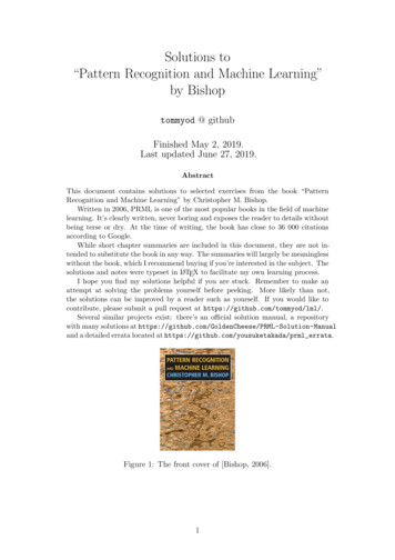
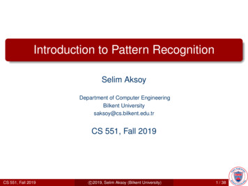
Other TopologiesThe back-propagation procedure is notlimited to feed-forward cascades.It can be applied to networks of modulewith any topology, as long as theconnection graph is acyclic.If the graph is acyclic (no loops) then, wecan easily find a suitable order in which tocall the fprop method of each module.The bprop methods are called in thereverse order.if the graph has cycles (loops) we have aso-called recurrent network. This will bestudied in a subsequent lecture.Y. LeCun: Machine Learning and Pattern Recognition – p. 5/3

More ModulesA rich repertoire of learning machines can be constructed with just a few module typesin addition to the linear, sigmoid, and euclidean modules we have already seen.We will review a few important modules:The branch/plus moduleThe switch moduleThe Softmax moduleThe logsum moduleY. LeCun: Machine Learning and Pattern Recognition – p. 6/3

The Branch/Plus ModuleThe PLUS module: a module with K inputsX1 , . . . , XK (of any type) that computes the sumof its inputs:Xout XXkkback-prop: E Xk E Xout kThe BRANCH module: a module with one inputand K outputs X1 , . . . , XK (of any type) thatsimply copies its input on its outputs:Xk Xin k [1.K]back-prop: E in P Ek XkY. LeCun: Machine Learning and Pattern Recognition – p. 7/3

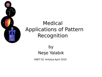
The Switch ModuleA module with K inputs X1 , . . . , XK (ofany type) and one additionaldiscrete-valued input Y .The value of the discrete input determineswhich of the N inputs is copied to theoutput.Xout Xδ(Y k)Xkk E E δ(Y k) Xk Xoutthe gradient with respect to the output iscopied to the gradient with respect to theswitched-in input. The gradients of all otherinputs are zero.Y. LeCun: Machine Learning and Pattern Recognition – p. 8/3

The Logsum Modulefprop:XoutX1 logexp( βXk )βkbprop: Eexp( βXk ) EP Xk Xout j exp( βXj )or E E Pk Xk Xoutwithexp( βXk )Pk Pj exp( βXj )Y. LeCun: Machine Learning and Pattern Recognition – p. 9/3

Log-Likelihood Loss function and Logsum ModulesiiiiMAP/MLE Loss Lll (W, Y , X ) E(W, Y , X ) 1βlogPiexp( βE(W,k,X))kA classifier trained with theLog-Likelihood loss can betransformed into an equivalentmachine trained with the energyloss.The transformed machine containsmultiple “replicas” of the classifier,one replica for the desired output,and K replicas for each possiblevalue of Y .Y. LeCun: Machine Learning and Pattern Recognition – p. 10/3

Softmax ModuleA single vector as input, and a “normalized” vector as output:exp( βxi )(Xout )i Pk exp( βxk )Exercise: find the bprop (Xout )i ? xjY. LeCun: Machine Learning and Pattern Recognition – p. 11/3

Radial Basis Function Network (RBF Net)Linearly combined Gaussianbumps.F (X, W, U ) P2i ui exp( ki (X Wi ) )The centers of the bumps can beinitialized with the K-meansalgorithm (see below), andsubsequently adjusted with gradientdescent.This is a good architecture for regression and function approximation.Y. LeCun: Machine Learning and Pattern Recognition – p. 12/3

MAP/MLE Loss and Cross-Entropyclassification (y is scalar and discrete). Let’s denote E(y, X, W ) Ey (X, W )MAP/MLE Loss Function:PX11 Xi[Eyi (X , W ) logexp( βEk (X i , W ))]L(W ) P i 1βkThis loss can be written asPexp( βEyi (X i , W ))1 X 1L(W ) log Pi , W ))P i 1 βexp( βE(XkkY. LeCun: Machine Learning and Pattern Recognition – p. 13/3

Cross-Entropy and KL-Divergenceilet’s denote P (j X , W ) i))Pexp( βEj (X ,W,ik exp( βEk (X ,W ))thenP1 X11L(W ) logP i 1 βP (y i X i , W )PDk (y i )1 X1XiDk (y ) logL(W ) P i 1 βP (k X i , W )kwith Dk (y i ) 1 iff k y i , and 0 otherwise.example1: D (0, 0, 1, 0) and P (. Xi , W ) (0.1, 0.1, 0.7, 0.1). with β 1,Li (W ) log(1/0.7) 0.3567example2: D (0, 0, 1, 0) and P (. Xi , W ) (0, 0, 1, 0). with β 1,Li (W ) log(1/1) 0Y. LeCun: Machine Learning and Pattern Recognition – p. 14/3

Cross-Entropy and KL-DivergenceP1 X1XDk (y i )iL(W ) Dk (y ) logP i 1 βP (k X i , W )kL(W ) is proportional to the cross-entropy between the conditional distributionof y given by the machine P (k X i , W ) and the desired distribution over classesfor sample i, Dk (y i ) (equal to 1 for the desired class, and 0 for the otherclasses).The cross-entropy also called Kullback-Leibler divergence between twodistributions Q(k) and P (k) is defined as:XkQ(k)Q(k) logP (k)It measures a sort of dissimilarity between two distributions.the KL-divergence is not a distance, because it is not symmetric, and it does notsatisfy the triangular inequality.Y. LeCun: Machine Learning and Pattern Recognition – p. 15/3

Multiclass Classification and KL-DivergenceAssume that our discriminant module F (X, W )produces a vector of energies, with one energyEk (X, W ) for each class.A switch module selects the smallest Ek to performthe classification.As shown above, the MAP/MLE loss below be seenas a KL-divergence between the desired distributionfor y, and the distribution produced by the machine.PX1 X1iL(W ) [Eyi (X , W ) logexp( βEk (X i , W ))]P i 1βkY. LeCun: Machine Learning and Pattern Recognition – p. 16/3

Multiclass Classification and SoftmaxThe previous machine: discriminant function with oneoutput per class switch, with MAP/MLE lossIt is equivalent to the following machine: discriminantfunction with one output per class softmax switch log lossP1 X1L(W ) log P (y i X, W )P i 1 βiwith P (j X , W ) the Ej ’s).i))Pexp( βEj (X ,Wik exp( βEk (X ,W ))(softmax ofMachines can be transformed into various equivalentforms to factorize the computation in advantageousways.Y. LeCun: Machine Learning and Pattern Recognition – p. 17/3

Multiclass Classification with a Junk CategorySometimes, one of the categories is “none of the above”, how can we handlethat?We add an extra energy wire E0 for the “junk” category which does not dependon the input. E0 can be a hand-chosen constant or can be equal to a trainableparameter (let’s call it w0 ).everything else is the same.Y. LeCun: Machine Learning and Pattern Recognition – p. 18/3

NN-RBF Hybridssigmoid units are generally moreappropriate for low-level featureextraction.Euclidean/RBF units are generally moreappropriate for final classifications,particularly if there are many classes.Hybrid architecture for multiclass classification: sigmoids below, RBFs on top softmax log loss.Y. LeCun: Machine Learning and Pattern Recognition – p. 19/3

Parameter-Space TransformsReparameterizing the function by transforming the spaceE(Y, X, W ) E(Y, X, G(U ))gradient descent in U space:U U ′ E(Y,X,W )η G U W′equivalent to the following algorithm in Wspace: W W G G ′ E(Y,X,W )η U U W′dimensions: [Nw Nu ][Nu Nw ][Nw ]Y. LeCun: Machine Learning and Pattern Recognition – p. 20/3

Parameter-Space Transforms: Weight SharingA single parameter is replicated multipletimes in a machineE(Y, X, w1 , . . . , wi , . . . , wj , . . .) E(Y, X, w1 , . . . , uk , . . . , uk , . . .)gradient: E() uk E() wi E() wjwi and wj are tied, or equivalently, uk isshared between two locations.Y. LeCun: Machine Learning and Pattern Recognition – p. 21/3

Parameter Sharing between ReplicasWe have seen this before: a parameter controlsseveral replicas of a machine.E(Y1 , Y2 , X, W ) E1 (Y1 , X, W ) E1 (Y2 , X, W )gradient: E(Y1 ,Y2 ,X,W ) W E1 (Y1 ,X,W ) W E1 (Y2 ,X,W ) WW is shared between two (or more) instances ofthe machine: just sum up the gradient contributions from each instance.Y. LeCun: Machine Learning and Pattern Recognition – p. 22/3

Path Summation (Path Integral)One variable influences the output through several othersE(Y, X, W ) E(Y, F1 (X, W ), F2 (X, W ), F3 (X, W ), V )P Ei (Y,Si ,V ) Fi (X,W ))gradient: E(Y,X,W i X Si XP Ei (Y,Si ,V ) Fi (X,W ) E(Y,X,W )gradient: i W Si Wthere is no need to implement these rules explicitely. They come out naturally of the objectoriented implementation.Y. LeCun: Machine Learning and Pattern Recognition – p. 23/3

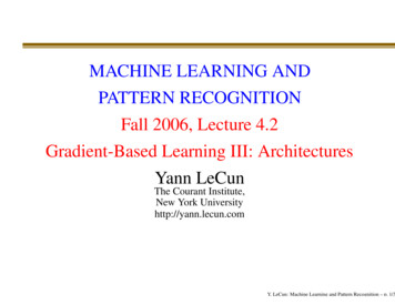
Mixtures of ExpertsSometimes, the function to be learned is consistent in restricted domains of the inputspace, but globally inconsistent. Example: piecewise linearly separable function.Solution: a machine composed of several“experts” that are specialized on subdomains ofthe input space.The output is a weighted combination of theoutputs of each expert. The weights are producedby a “gater” network that identifies whichsubdomain the input vector is in.PF (X, W ) k uk F k (X, W k ) withuk 0Pexp( βGk (X,W ))0k exp( βGk (X,W ))the expert weights uk are obtained by softmax-ingthe outputs of the gater.example: the two experts are linear regressors, thegater is a logistic regressor.Y. LeCun: Machine Learning and Pattern Recognition – p. 24/3

Sequence Processing: Time-Delayed InputsThe input is a sequence of vectors Xt .simple idea: the machine takes a timewindow as inputR F (Xt , Xt 1 , Xt 2 , W )Examples of use:predict the next sample in a timeseries (e.g. stock market, waterconsumption)predict the next character or word in atextclassify an intron/exon transition in aDNA sequenceY. LeCun: Machine Learning and Pattern Recognition – p. 25/3

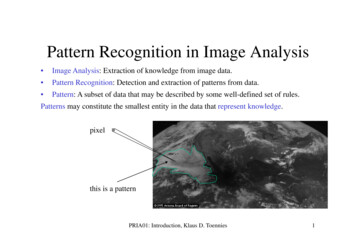
Sequence Processing: Time-Delay NetworksOne layer produces a sequence for the next layer: stacked time-delayed layers.layer1 Xt1 F 1 (Xt , Xt 1 , Xt 2 , W 1 )11, W 2), Xt 2layer2 Xt2 F 1 (Xt1 , Xt 1cost Et C(Xt1 , Yt )Examples:predict the next sample in a time series withlong-term memory (e.g. stock market, waterconsumption)recognize spoken wordsrecognize gestures and handwrittencharacters on a pen computer.How do we train?Y. LeCun: Machine Learning and Pattern Recognition – p. 26/3