WIXLIB

91.2. OPERATIONS ON SETSIn the recursive definition of a set, the first rule is the basis of recursion, the second rule givesa method to generate new element(s) from the elements already determined and the third rulebinds or restricts the defined set to the elements generated by the first two rules. The third ruleshould always be there. But, in practice it is left implicit. At this stage, one should make itexplicit.Definition 1.1.4. Let X and Y be two sets.1. Suppose X is the set such that whenever x X, then x Y as well. Here, X is said to be asubset of the set Y , and is denoted by X Y . When there exists x X such that x 6 Y , thenwe say that X is not a subset of Y ; and we write X 6 Y .2. If X Y and Y X, then X and Y are said to be equal, and is denoted by X Y .3. If X Y and X 6 Y , then X is called a proper subset of Y .Thus, X is a proper subset of Y if and only if X Y and X 6 Y .Example 1.1.5.1. For any set X, we see that X X. Thus, . Also, X. Hence, theempty set is a subset of every set. It thus follows that there is only one empty set.2. We know that N W Z Q R C.3. Note that 6 .4. Let X {a, b, c}. Then a X but {a} X. Also, {{a}} 6 X.5. Notice that {{a}} 6 {a} and {a} 6 {{a}}; though {a} {a, {a}} and also {a} {a, {a}}.Operations on setsDR1.2AFTWe now mention some set operations that enable us in generating new sets from existing ones.Definition 1.2.1. Let X and Y be two sets.1. The union of X and Y , denoted by X Y , is the set that consists of all elements of X and alsoall elements of Y . More specifically, X Y {x x X or x Y }.2. The intersection of X and Y , denoted by X Y , is the set of all common elements of X andY . More specifically, X Y {x x X and x Y }.3. The sets X and Y are said to be disjoint if X Y .Example 1.2.2.1. Let A {1, 2, 4, 18} and B {x : x is an integer, 0 x 5}. Then,A B {1, 2, 3, 4, 5, 18} and A B {1, 2, 4}.2. Let S {x R : 0 x 1} and T {x R : .5 x 7}. Then,S T {x R : 0 x 7} and S T {x R : .5 x 1}.3. Let X {{b, c}, {{b}, {c}}, b} and Y {a, b, c}. ThenX Y {b} and X Y {a, b, c, {b, c}, {{b}, {c}} }.We now state a few properties related to the union and intersection of sets.Lemma 1.2.3. Let R, S and T be sets. Then,1. (a) S T T S and S T T S (union and intersection are commutative operations).

10CHAPTER 1. BASIC SET THEORY(b) R (S T ) (R S) T and R (S T ) (R S) T (union and intersection areassociative operations).(c) S S T, T S T .(d) S T S, S T T .(e) S S, S .(f ) S S S S S.2. Distributive laws (combines union and intersection):(a) R (S T ) (R S) (R T ) (union distributes over intersection).(b) R (S T ) (R S) (R T ) (intersection distributes over union).Proof. 2a. Let x R (S T ). Then, x R or x S T . If x R then, x R S and x R T .Thus, x (R S) (R T ). If x 6 R, then x S T . So, x S and x T . Here, x R S andx R T . Thus, x (R S) (R T ). In other words, R (S T ) (R S) (R T ).Now, let y (R S) (R T ). Then, y R S and y R T . Now, if y R S then eithery R or y S or both.If y R, then y R (S T ). If y 6 R then the conditions y R S and y R T imply that y Sand y T . Thus, y S T and hence y R (S T ). This shows that (R S) (R T ) R (S T ),and thereby proving the first distributive law. The remaining proofs are left as exercises.Exercise 1.2.4.1. Complete the proof of Lemma 1.2.3.(a) S (S T ) S (S T ) S.DR(b) S T if and only if S T T .AFT2. Prove the following:(c) If R T and S T then R S T .(d) If R S and R T then R S T .(e) If S T then R S R T and R S R T .(f ) If S T 6 then either S 6 or T 6 .(g) If S T 6 then both S 6 and T 6 .(h) S T if and only if S T S T .Definition 1.2.5. Let X and Y be two sets.1. The set difference of X and Y , denoted by X \ Y , is defined by X \ Y {x X : x 6 Y }.2. The set (X \ Y ) (Y \ X), denoted by X Y , is called the symmetric difference of X and Y .Example 1.2.6.1. Let A {1, 2, 4, 18} and B {x Z : 0 x 5}. Then,A \ B {18}, B \ A {3, 5} and A B {3, 5, 18}.2. Let S {x R : 0 x 1} and T {x R : 0.5 x 7}. Then,S \ T {x R : 0 x 0.5} and T \ S {x R : 1 x 7}.3. Let X {{b, c}, {{b}, {c}}, b} and Y {a, b, c}. ThenX \ Y {{b, c}, {{b}, {c}}}, Y \ X {a, c} and X Y {a, c, {b, c}, {{b}, {c}}}.

111.3. RELATIONSIn naive set theory, all sets are essentially defined to be subsets of some reference set, referred toas the universal set, and is denoted by U . We now define the complement of a set.Definition 1.2.7. Let U be the universal set and X U . Then, the complement of X, denoted byX c , is defined by X c {x U : x 6 X}.We state more properties of sets.Lemma 1.2.8. Let U be the universal set and S, T U . Then,1. U c and c U .2. S S c U and S S c .3. S U U and S U S.4. (S c )c S.5. S S c if and only if S .6. S T if and only if T c S c .7. S T c if and only if S T and S T U .8. S \ T S T c and T \ S T S c .9. S T (S T ) \ (S T ).AF(b) (S T )c S c T c .DR(a) (S T )c S c T c .T10. De-Morgan’s Laws:The De-Morgan’s laws help us to convert arbitrary set expressions into those that involve onlycomplements and unions or only complements and intersections.Exercise 1.2.9. Let S and T be subsets of a universal set U .1. Then prove Lemma 1.2.8.2. Suppose that S T T . Is S ?Definition 1.2.10. Let X be a set. Then, the set that contains all subsets of X is called the powerset of X and is denoted by P(X) or 2X .Example 1.2.11.1. Let X . Then P( ) P(X) { , X} { }.2. Let X { }. Then P({ }) P(X) { , X} { , { }}.3. Let X {a, b, c}. Then P(X) { , {a}, {b}, {c}, {a, b}, {a, c}, {b, c}, {a, b, c}}.4. Let X {{b, c}, {{b}, {c}}}. Then P(X) { , {{b, c}}, {{{b}, {c}}}, {{b, c}, {{b}, {c}}} }.1.3RelationsIn this section, we introduce the set theoretic concepts of relations and functions. We will use theseconcepts to relate different sets. This method also helps in constructing new sets from existing ones.

12CHAPTER 1. BASIC SET THEORYDefinition 1.3.1. Let X and Y be two sets. Then their Cartesian product, denoted by X Y , isdefined as X Y {(a, b) : a X, b Y }. The elements of X Y are also called ordered pairswith the elements of X as the first entry and elements of Y as the second entry. Thus,(a1 , b1 ) (a2 , b2 ) if and only if a1 a2 and b1 b2 .Example 1.3.2.1. Let X {a, b, c} and Y {1, 2, 3, 4}. ThenX X {(a, a), (a, b), (a, c), (b, a), (b, b), (b, c), (c, a), (c, b), (c, c)}.X Y {(a, 1), (a, 2), (a, 3), (a, 4), (b, 1), (b, 2), (b, 3), (b, 4), (c, 1), (c, 2), (c, 3), (c, 4)}.2. The Euclidean plane, denoted by R2 R R {(x, y) : x, y R}.3. By convention, Y X . In fact, X Y if and only if X or Y .Remark 1.3.3. Let X and Y be two nonempty sets. Then, X Y can also be defined as follows:Let x X and y Y and think of (x, y) as the set {{x}, {x, y}}, i.e., we have a new set in which anelement (a set formed using the first element of the ordered pair) is a subset of the other element (a setformed with both the elements of the ordered pair). Then, with the above understanding, the orderedpair (y, x) will correspond to the set {{y}, {x, y}}. As the two sets {{x}, {x, y}} and {{y}, {x, y}} arenot the same, the ordered pair (x, y) 6 (y, x).Exercise 1.3.4. Let X, Y, Z and W be nonempty sets. Then, prove the following statements:AFT1. The product construction can be used on sets several times, e.g.,DRX Y Z {(x, y, z) : x X, y Y, z Z} (X Y ) Z X (Y Z).2. X (Y Z) (X Y ) (X Z).3. X (Y Z) (X Y ) (X Z).4. (X Y ) (Z W ) (X Z) (Y W ).5. (X Y ) (Z W ) (X Z) (Y W ). Give an example to show that the converse need notbe true.6. Is it possible to write the set T {(x, x, y) : x, y N} as Cartesian product of 3 sets? Whatabout the the set T {(x, x2 , y) : x, y N}?A relation can be informally thought of as a property which either holds or does not hold betweentwo objects. For example, x is taller than y can be a relation. However, if x is taller than y, then ycannot be taller than x.Definition 1.3.5. Let X and Y be two nonempty sets. A relation R from X to Y is a subset ofX Y , i.e., it is a collection of certain ordered pairs. We write xRy to mean (x, y) R X Y .Thus, for any two sets X and Y , the sets and X Y are always relations from X to Y . A relationfrom X to X is called a relation on X.Example 1.3.6.1. Let X be any nonempty set and consider the set P(X). Define a relation Ron P(X) by R {(S, T ) P(X) P(X) : S T }.2. Let A {a, b, c, d}. Some relations R on A are:(a) R A A.

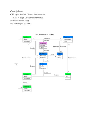
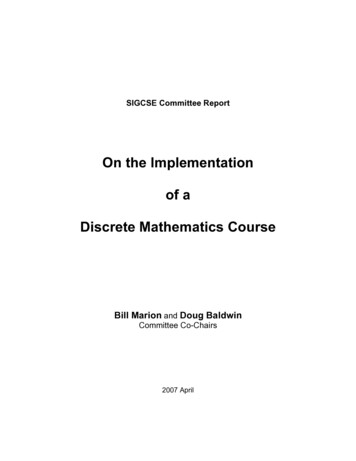
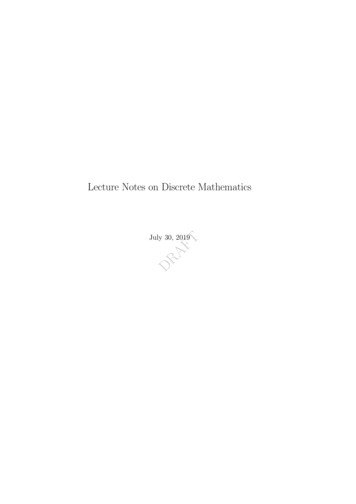
131.3. RELATIONS(b) R {(a, a), (b, b), (c, c), (d, d), (a, b), (a, c), (b, c)}.(c) R {(a, a), (b, b), (c, c)}.(d) R {(a, a), (a, b), (b, a), (b, b), (c, d)}.(e) R {(a, a), (a, b), (b, a), (a, c), (c, a), (c, c), (b, b)}.(f) R {(a, b), (b, c), (a, c), (d, d)}.(g) R {(a, a), (b, b), (c, c), (d, d), (a, b), (b, c)}.(h) R {(a, a), (b, b), (c, c), (d, d), (a, b), (b, a), (b, c), (c, b)}.(i) R {(a, a), (b, b), (c, c), (a, b), (b, c)}.Sometimes, we draw pictures to have a better understanding of different relations. For example,to draw pictures for relations on a set X, we first put a node for each element x X and labelit x. Then, for each (x, y) R, we draw a directed line from x to y. If (x, x) R then a loop isdrawn at x. The pictures for some of the relations is given in Figure 1.1.dcdcdabababAFTcExample 2.bExample 2.cDRA AFigure 1.1: Pictorial representation of some relations from Example 23. Let A {1, 2, 3}, B {a, b, c} and let R {(1, a), (1, b), (2, c)}. Figure 1.2 represents therelation R. 11a2b3cRFigure 1.2: Pictorial representation of the relation in Example 34. Let R {(x, y) : x, y Z and y x 5m for some m Z} is a relation on Z. If we try to drawa picture for this relation then there is no arrow between any two elements of {1, 2, 3, 4, 5}.5. Fix n N. Let R {(x, y) : x, y Z and y x nm for some m Z}. Then, R is a relationon Z. A picture for this relation has no arrow between any two elements of {1, 2, 3, . . . , n}.1We use pictures to help our understanding and they are not parts of proof.

14CHAPTER 1. BASIC SET THEORYDefinition 1.3.7. Let X and Y be two nonempty sets and let R be a relation from X to Y . Then,the inverse relation, denoted by R 1 , is a relation from Y to X, defined by R 1 {(y, x) Y X :(x, y) R}. So, for all x X and y Y(x, y) R if and only if (y, x) R 1 .Example 1.3.8.1. If R {(1, a), (1, b), (2, c)} then R 1 {(a, 1), (b, 1), (c, 2)}.2. Let R {(a, b), (b, c), (a, c)} be a relation on A {a, b, c} then R 1 {(b, a), (c, b), (c, a)} isalso a relation on A.Let R be a relation from X to Y . Consider an element x X. It is natural to ask if there existsy Y such that (x, y) R. This gives rise to the following three possibilities:1. (x, y) 6 R for all y Y .2. There is a unique y Y such that (x, y) R.3. There exists at least two elements y1 , y2 Y such that (x, y1 ), (x, y2 ) R.One can ask similar questions for an element y Y . To accommodate all these, we introduce anotation in the following definition.Definition 1.3.9. Let R be a nonempty relation from X to Y . Then,1. the set dom R: {x : (x, y) R} is called the domain of R1 , and2. the set rng R: {y Y : (x, y) R} is called the range of R.TNotation 1.3.10. Let R be a nonempty relation from X to Y . Then,AF1. for any set Z, one writes R(Z) : {y : (z, y) R for some z Z}.DR2. for any set W , one writes R 1 (W ) : {x X : (x, w) R for some w W }.Example 1.3.11. Let a, b, c, and d be distinct symbols and let R {1, a), (1, b), (2, c)}. Then,1. dom R {1, 2}, rng R {a, b, c},2. R({1}) {a, b}, R({2}) {c}, R({1, 2}) {a, b, c}, R({1, 2, 3}) {a, b, c}, R({4}) .3. dom R 1 {a, b, c}, rng R 1 {1, 2},4. R 1 ({a}) {1}, R 1 ({a, b}) {1}, R 1 ({b, c}) {1, 2}, R 1 ({a, d}) {1}, R 1 ({d}) .The following is an immediate consequence of the definition, but we give the proof of a few partsfor the sake of better understanding.Proposition 1.3.12. Let R be a nonempty relation from X to Y , and let Z be any set.1. R(Z) R(X Z) Y, R 1 (Z) R 1 (Z Y ) X.2. dom R R 1 (Y ) rng R 1 X, rng R R(X) dom R 1 Y.3. R(Z) 6 if and only if dom R Z 6 .4. R 1 (Z) 6 if and only if rng R Z 6 .Proof. We prove the last two parts. The proof of the first two parts is left as an exercise.3. Let f (S) 6 . There exist a S A and b B such that (a, b) f . It implies that a dom f S(a S). Converse is proved in a similar way.4. Let rng f S 6 . There exist b rng f S and a A such that (a, b) f . Then a f 1 (b) f 1 (S). Similarly, the converse follows.1In some texts, the set X is referred to as the domain set of R and it should not be confused with dom R.

151.4. FUNCTIONS1.4FunctionsDefinition 1.4.1. Let X and Y be nonempty sets and let f be a relation from X to Y .1. f is called a partial function from X to Y , denoted by f : X * Y , if for each x X, f ({x})is either a singleton or .2. For an element x X, if f ({x}) {y}, a singleton, we write f (x) y. Hence, y is referred toas the image of x under f ; and x is referred to as the pre-image of y under f .f (x) is said to be undefined at x X if f ({x}) .3. If f is a partial function from X to Y such that for each x X, f ({x}) is a singleton then f iscalled a function and is denoted by f : X Y .Observe that for any partial function f : X * Y , the condition (a, b), (a, b0 ) f implies b b0 .Thus, if f : X * Y , then for each x X, either f (x) is undefined, or there exists a unique y Ysuch that f (x) y. Moreover, if f : X Y is a function, then f (x) exists for each x X, i.e., thereexists a unique y Y such that f (x) y.It thus follows that a partial function f : X * Y is a function if and only if dom f X, i.e.,domain set of f is X.Example 1.4.2. Let A {a, b, c, d}, B {1, 2, 3, 4} and X {3, 4, b, c}.1. Consider the relation R1 {(a, 1), (b, 1), (c, 2)} from A to B. The following are true.(a) R1 is a partial function.(c) R1 (X) {1, 2}.AFT(b) R1 (a) 1, R1 (b) 1, R1 (c) 2. Also, R1 ({d}) ; thus R1 (d) is undefined.DR(d) R1 1 {(1, a), (1, b), (2, c)}. So, R1 1 ({1}) {a, b} and R1 1 (2) c. For any x X,R1 1 (x) . Therefore, R1 1 (x) is undefined.2. R2 {(a, 1), (b, 4), (c, 2), (d, 3)} is a relation from A to B. The following are true.(a) R2 is a partial function.(b) R2 (a) 1, R2 (b) 4, R2 (c) 2 and R2 (d) 3.(c) R2 (X) {2, 4}.(d) R2 1 (1) a, R2 1 (2) c, R2 1 (3) d and R2 1 (4) b. Also, R2 1 (X) {b, d}.Convention:Let p(x) be a polynomial in the variable x with integer coefficients. Then, by writing ‘f : Z Zis a function defined by f (x) p(x)’, we mean the function f {(a, p(a)) : a Z}. For example,the function f : Z Z given by f (x) x2 corresponds to the set {(a, a2 ) : a Z}.Example 1.4.3.1. For A {a, b, c, d} and B {1, 3, 5}, let f {(a, 5), (b, 1), (d, 5)} be a relationin A B. Then, f is a partial function with dom f {a, b, d} and rng f {1, 5}. Further, wecan define a function g : {a, b, d} {1, 5} by g(a) 5, g(b) 1 and g(d) 5. Also, using g, oneobtains the relation g 1 {(1, b), (5, a), (5, d)}.2. The following relations f : Z Z are indeed functions.(a) f {(x, 1) : x is even} {(x, 5) : x is odd}.(b) f {(x, 1) : x Z}.(c) f {(x, 1) : x 0} {(0, 0)} {(x, 1) : x 0}.

16CHAPTER 1. BASIC SET THEORY3. Define f : Q N by f {( pq , 2p 3q ) : p, q N, q 6 0, p and q are coprime}. Then, f is afunction.Remark 1.4.4.1. If X , then by convention, one assumes that there is a function, called theempty function, from X to Y .2. If Y and X 6 , then by convention, we say that there is no function from X to Y .3. Individual relations and functions are also sets. Therefore, one can have equality between relations and functions, i.e., they are equal if and only if they contain the same set of pairs. For example, let X { 1, 0, 1}. Then, the functions f, g, h : X X defined by f (x) x, g(x) x x andh(x) x3 are equal as the three functions correspond to the relation R {( 1, 1), (0, 0), (1, 1)}on X.4. A function is also called a map.5. Throughout the book, whenever the phrase ‘let f : X Y be a function’ is used, it will beassumed that both X and Y are nonempty sets.Some important functions are now defined.Definition 1.4.5. Let X be a nonempty set.1. The relation Id : {(x, x) : x X} is called the identity relation on X.2. The function f : X X defined by f (x) x, for all x X, is called the identity function andis denoted by Id.1. Do the following relations represent functions? Why?DRExercise 1.4.6.AFT3. The function f : X R with f (x) 0, for all x X, is called the zero function and is denotedby 0.(a) f : Z Z defined byi. f {(x, 1) : 2 divides x} {(x, 5) : 3 divides x}.ii. f {(x, 1) : x S} {(x, 1) : x S c }, where S {n2 : n Z} and S c Z \ S.iii. f {(x, x3 ) : x Z}. (b) f : R R defined by f {(x, x) : x R }, where R is the set of all positive realnumbers. (c) f : R R defined by f {(x, x) : x R}. (d) f : R C defined by f {(x, x) : x R}.(e) f : R R defined by f {(x, loge x ) : x R }, where R is the set of all negative realnumbers.(f ) f : R R defined by f {(x, tan x) : x R}.2. Let f : X Y b

DRAFT 1.2. OPERATIONS ON SETS 9 In the recursive de nition of a set, the rst rule is the basis of recursion, the second rule gives a method to generate new element(s) from the elements already determined and the third rule