Transcription
Math 563 Lecture NotesThe discrete Fourier transformSpring 2020The point: A brief review of the relevant review of Fourier series; introduction to the DFTand its good properties (spectral accuracy) and potential issues (aliasing, error from lackof smoothness). There are a vast number of sub-topics and applications that could be discussed; a few examples are included at the end (we’ll likely make use of the DFT again laterin solving differential equations).Related reading: Details on the DFT can be found in Quarteroni, . Many other sourceshave good descriptions of the DFT as well (it’s an important topic), but beware of slightlydifferent notation. Reading the documentation for numpy or Matlab’s fft is suggested aswell, to see how the typical software presents the transform for practical use.1Fourier series (review/summary)We consider functions in L2 [0, 2π] (with weight w(x) 1), which have a Fourier seriesf Xikxck ek ,1ck 2πZ2πf (x)e ikx dx.0The basis functions φk eikx are orthogonal in the inner product hf, gi R 2π0f (x)g(x) dx.In this section, the space L2 [0, 2π] is regarded as the space of 2π-periodic functions, i.e.functions defined for x R that satisfyf (x) f (x 2π) for all x.By this property, the function is defined by its values on one period, so it suffices to considerthe function on the interval [0, 2π]. The main point is that continuity of the periodic functionrequires that the endpoints match:f continuous in [0, 2π] and f (0) f (2π).The same goes for differentiability. The ‘periodic’ definition is key, as error properties willdepend on the smoothness of f as a periodic function.1
If f is real-valued, it is not hard to show thatc k ck .Writing the coefficients as cn 12 (ak ibk ) we have (by grouping k and k terms) a0 X f (x) an cos kx bn sin kx2k 1which is the Fourier series in real form. Two standard examples of Fourier series:(1x 0square wave: fS (x) ,x [ π, π] 1 x 0triangle wave: fT (x) x ,x [ π, π](1)(2)3.5312.50.521.501-0.50.50-1-20-5205The Fourier series for the square wave is straightforward to calculate:4 X 1fS (x) sin nxπ n odd nor 4X 1fS (x) sin((2n 1)x).π n 1 2n 1Similar to the square wave, we get for the triangle wave that 11 4XfT (x) cos((2n 1)x).2 π n 1 (2n 1)2Convergence: The partial sums of the Fourier series are least-squares approximations withrespect to the given basis. In particular, if f is real thenlim kf SN k2 0,N SN : NXNck ek N2ikxa0 X ak cos kx bk sin kx.2k 1
More can be said about the coefficients; by integrating the formula for ck by parts we canobtain the following bounds:These bounds, coupled with Parseval’s theorem, connect the convergence rate of the series to the smoothness of f as a periodic function.The Fourier series allows for some discontinuities. Definef (x ) lim f (ξ),f (x ) lim f (ξ).ξ%xξ&xTheorem (Pointwise/uniform convergence): Let SN (x) be the N -th partial sum of theFourier series for f L2 [ , ]. If f and f 0 are piecewise continuous, then(f (x)if f is continuous at xlim SN (x) f (x) : 1 N (f (x ) f (x )) if f has a jump at x.2That is, the partial sums converge pointwise to the average of the left and right limits.Near a discontinuity x0 , one has Gibbs’ phenomenon, where the series fails to convergeuniformly, leaving a maximum error near x0 of about 9% of the discontinuity (evident in thesquare wave example above).1.1Decay of Fourier coefficientsConsider L2 functions in [0, 2π] and the Fourier series a0 Xan cos nx bn sin nx. f (x) 2n 1Worst case: Suppose f as a periodic function is piecewise continuous but has a jump (e.g.the square wave). Thenan , bn O(1/n).This is enough to get norm convergence:2kf SN k const. · X(a2n b2n ) O(1/N ).n N 1However, 1/n decay is not enough to get convergence at each point (P1/n diverges).Nicer case: However, if the function is smoother then we can do better. If f L2 [ π, π]and its derivatives up to f (p 1) are continuous as periodic functions and f (p) is continuousexcept at a set of jumps then, for some constant C, an C,np 1 bn 3C.np 1
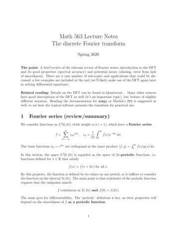
10 -23.5310 -32.5210 -41.5110 -50.5010 -202FigureR 1: Partial sums for the triangle/square wave and log-log plot of the squared L2πerror π SN (x) f (x) 2 dx. For the triangle, cn 1/n2 and the error decreases likeP P 22 23n N (1/n) 1/N.n N (1/n ) 1/N . For the square, cn 1/n; the error decreases asThus, in general, smoother f faster convergence of its Fourier series. Informally, weget one factor of 1/n for each derivative (as a periodic function), starting with the 0-th andending with the first one that has a jump. For the square/triangle:square jump in f cn 1/ntri. f cts. jump in f 0 cn 1/n2 .Smooth functions: If the function f (x) is smooth and 2π-periodic (derivatives of allorders), the the coefficients have the exponential bound an e αnwhere α (The decay rate) is the distance from [0, 2π] to the nearest singularity of the functionin the complex plane. That is, less singular functions have coefficients that decay faster.4
Informal definition: When an error has a bound of the formkf f n k Cn p if f C p ,kf f n k Ce an if f C we say the approximation has spectral accuracy. That is, the error behaves like theFourier series error (you will sometimes see this referred to as exponential type). We havealready seen that the trapezoidal rule, for instance, has spectral accuracy while a splineapproximation does not.The benefit (and disadvantage, sometimes) of the property is that the smoothnessof f determines the convergence rate. When f is smooth, this is great; when f is notsmooth, the lack of smoothness can be a problem.2The discrete Fourier transform2.1Getting to the discrete form: using the trapezoidal ruleWe know from the previous theory that the partial sums are best approximations in theleast-squares sense (minimizing the error in the L2 norm):g SN NXck eikx minimizes kf gk2 for functions of the form g NX(· · · )eikx .k Nk NComputing the coefficients ck requires estimating the integral.As we will see, the trapezoidal rule is the right choice. Let xj jh with h 2π/N .Assume that f is periodic and continuous, so f0 fN . Using the trapezoidal rule,Z 2π1ck f (x)e ikx dx2π 0!N 1h f0 fN X fj e ikxj2π 22j 1N 11 Xfj e ikhj N j 0 N 11 Xfj e 2πikj/NN j 0The transformation from fj to ck is the discrete Fourier transform:N 1{fj }j 0 N 11 XFk fj e 2πikj/N .N j 0 1{Fk }Nk 0 ,5
We may then use this transform to estimate partial sums of the Fourier series (the leastsquares approximation to f ) using data at equally spaced points.Note that if f is real and m N/2 then, writing Fk (ak ibk )/2,f (x) mXmikxFk ek ma0 X ak cos kx bk sin kx 2k 1(3)where, from the identity eiN xj 1,ck cN k for k 0.In this way the DFT {ck } is ‘cyclic’ (it wraps around for indices past N ). Note that theDFT approximation (3) is not quite the Fourier series partial sum, because the Fk ’sare not equal to the Fourier series coefficients (but they are close!).To get a better understanding, we should be more careful; at present, it is not clear why thetrapezoidal rule should be used for the integral.2.2The discrete form (from discrete least squares)Instead, we derive the transform by considering ‘discrete’ approximation from data. Letx0 , · · · , xN be equally spaced nodes in [0, 2π] and suppose the function data is given at thenodes. Remarkably, the basis {eikx } is also orthogonal in the discrete inner producthf, gid N 1Xf (xj )g(xj ).j 0Precisely, for integers j, k we have(0 if j 6 kheijx , eikx id N if j k.The general theory for least-squares approximation then applies (see HW). For ease of notation, the Fourier coefficients for f are denoted with a capital letter. It follows thatf mXk mikxFk e,N 1hf, eikx id1 XFk ikx ikx f (xj )e ikxjhe , e idN j 0which is exactly the discrete Fourier transform. Moreover, the orthogonality relation givesa formula for the inverse transform. The result is the following:6
Definition (Discrete Fourier transform): Suppose f (x) is a 2π-periodic function. Letxj jh with h 2π/N and fj f (xj ). The discrete Fourier transform of the data 1N 1{fj }Nj 0 is the vector {Fk }k 0 whereFk N 11 Xfj e 2πikj/NN j 0(4)and it has the inverse transformfj N 1XFk e2πikj/N .(5)k 0Letting ωN e 2πi/N , the transform and inverse can be written asFk N 11 Xjkfj ωN,N j 0fj N 1X jkFk ωN.j 0Proof. The inverse formula is not hard to prove; just use the definitions and the discreteorthogonality relation to calculateN 1XikxjFk e k 0 N 1 N 1XXk 0 m 0N 1N 1XXfmm 0 fm e ikxm eikxjN 1Xeik(xj xm )k 0fm heijx , eimx idm 0 N fj .2.3AliasingAs a simple (but subtle) example, considerf (x) cos 2x 2 sin 4x.The frequencies in this function are 2 (with coeffs. 1/2) and 4 (with coeffs. 2/i). TheDFT, therefore, should have peaks at these values of k.Consider taking N equally spaced samples (xj jh with h 2π/N and j 0, · · · , N 1)with N 6 and N 16 as shown below.7
20224602462020Since e16ixj 1 for all j, the frequencies 2 and 4 appear in the transform in the k 14and k 12 places (they ‘wrap around’ from zero to the other side of the array).The real/imaginary parts of the DFT are shown below, confirming that it works. Sincethe underlying function is real, it makes sense to ‘center’ the DFT by shifting the data byN/2 so that k 0 is in the center; the plot then has a nice (c)Im(c)0.51.01550k (shifted)5However, when N 6, the available frequencies are only k 0, 1, 2, 3. The DFT sees k 4as 2 and k 4 as 2 - as if the function were 2 sin 2x. There are not enough samplesto resolve the frequency, which causes it to ‘wrap back around’ and appear to be a differentvalue (this effect is called c)Im(c)0.51.0420k (shifted)2The example here suggests that the range of frequencies used in the DFT (the ‘bandwidth’)must be wide enough to fit the bandwidth of the function to avoid aliasing. In particular,the number of sample points N must be at least twice the largest frequency (the Nyquistsampling rate).8
2.4Real functions, interpolationDefinition A trigonometric polynomial of degree d is a polynomial in e ix of degree d,e.g. cos2 θ sin2 θ is a trig. polynomial of degree 2.The inverse formula (5) shows that the trigonometric polynomialpN (x) N 1XFk eikx(6)k 0satisfiespN (xj ) fj for j 0, · · · , N 1.Thus, it is a ‘trigonometric interpolant’ for the data (xj , fj ). However, there is a catch! Iff (x) is real, then pN (x) given by (6) may be complex (away from the interpolation points).When the function f (x) is real, we should instead ‘symmetrize’ the formula to constructa real-valued interpolant. Let N 2m be even. Observe that if x xj is a node thenpN (xj ) N 1XFk eikxjk 0N/2 XFk e2πijk/N k 0 N/2XFk e2πijk/Nk N/2 12πijk/NFk emX 1X k 0 N 1XFk N e2πijk/N(shift sum by N )k (N/2 1)F̃k eikxjk (m 1)m 1X k (m 1)whereF̃k eikxj F̃m iN xj /2 F̃m iN xj /2e e22(Fk NF̃k Fk1 N/2 k 0.0 k N/2F̃ k F̃k ,F̃m , F̃0 are real.(split into N/2 terms)One can check thatWriting F̃k 12 (ak bk i) and F̃m am , we therefore have an interpolant in the formm 1Xa0 ampN (x) cos mx ak cos kx bk sin kx.22k 19
Note that the k N/2 coefficient gets split into N/2 parts (it is aliased!) so it becomesboth halves of the cos mx term; it has no imaginary part so there is no sin mx term.Caution (uniqueness): Observe that the calculation shows that the interpolant is notunique; we are allowed to shift by various multiples in the exponent and still have theinterpolation property. The DFT can only distinguish frequencies k up to a multiple of N ;all functions ei(k pN )x are the same at the given data points for any integer p.2.5Example (interpolant)Consider the trigonometric interpolant forf (x) x(2π x),x [0, 2π]using the points 0, π/2, π, 3π/2 (so N 4). Note that 2π is also an interpolation point, butis equivalent to zero.In complex form, the interpolant isF2F2 2ixe F3 e ix F0 F1 eix e2ix .22p2 (x) All the F ’s are real here (check this!). Setting Fk ak /2 givesp(x) a0a2 a1 cos x cos 2x.22With more points, the approximation improves. To better understand the error, we can usethe Fourier series theory.1086420N 402x410864206N 2402x46Since f (x) (as a periodic function) is continuous but f 0 has a jump at x 0, the coefficientsdecay like 1/k 2 (see subsection 1.1). This suggests thatmax pN (x) f (x) x [0,2π]10Cas N N
which is indeed the case. The error is not exciting here, because the lack of differentiabilityat the endpoint causes trouble (on the other hand, if f is smooth and periodic, then theapproximation will be much better!).16max. errslope -11014210010Re(c)01248216 32 64 128N100k (shifted)10For a more dramatic example, suppose instead we interpolatef (x) x,x [0, 2π].The function is not continuous (with a jump x 0). Using the N points 0, 2π/N, · · · 2π(N 1)/N ) means the interpolant matches the function at x 0, but has the wrong behavior asx 2π (the interpolant must be continuous!).N 86N 32644220002x4602x46In addition, we observe Gibbs’ phenomnenon in the approximation; the effect of the discontinuity spoils the approximation nearby.To get around this, the standard solution is to use smoothing - the coefficients in theFourier series are ‘smoothed out’ by adding a numerical factor that improves the smoothness without changing the function much (see, for instance, Lanczos smoothing in thetextbook).1The result is true for Fourier series, as discussed. From the first derivation of the DFT, we saw that theFourier series and DFT approximation differ by a trapezoidal rule application. Thus, it’s plausible that theDFT inherits the same convergence properties as the Fourier series, which is more or less the case.11
2.6The Fast Fourier transform (the short version)The discrete Fourier transform has the formN 11 XkjFk fj ωNN j 0where ωN e 2πi/N . Each component takes O(N ) operations to compute and there are Ncomponents, so naively, evaluating the DFT takes O(N 2 ) operations.However, the coefficients in the sum are not arbitrary! They are powers of ω, and thatstructure can be exploited to save work. The idea is worth seeing to understand why it isfaster; the nasty implementation details are omitted here in favor of showing the idea.2Let ωN e 2πi/N and assume thatN 2M is a power of 2.The idea is to split the sum into ‘odd’ and ’even’ parts. We writeFk Sk Tkwhere (with the sum over indices in the range 0 to N 1)XXkjkjSk fj ω Nfj ωN, Tk j evenj oddSince N is even, the even sum can be written in terms of powers of ωN/2N/2 1Sk X 2πik(2m)/Nf2m e m 0N/2Xf2m (ωN/2 )kmm 0 Sk DF T ((f0 , f2 , · · · , fN 2 ))kand the odd sum can be written the same way, factoring one power of ω out:N/2 1Tk X 2πik(2m 1)/Nf2m 1 e 2πik/N em 0N/2Xf2m 1 (ωN/2 )kmm 0 Tk e 2πik/N DF T ((f1 , f3 , · · · , fN 1 ))kThe DFT therefore requires two DFTs of length N/2 for the odd/even parts O(N ) operations to combine the odd/even parts Tk and Sk (by addition)2Numerical Recipes, 3rd edition has a good description of the implementation details.12
This calculation defines a recursive process for computing the DFT. If N is a power of twothen log2 (N ) iterations of the process are required, so a length N DFT requires O(N log N )operations.The algorithm described here is a first version of the Fast Fourier transform. Threecomponents are missing: Proper handling of cases when N is not a power of 2 Mkaing the algorithm not use true recursion. By some clever encoding, one can writethe algorithm in a non-recursive way (using loops), which avoids overhead and allowsfor optimization. The ‘base case’ when N is small. One can go all the way to N 1 or 2; in practice itis most efficient to implement a super-efficient base case at certain values of N .The gain in efficiency is quite profound here - going from O(N 2 ) to O(N log N ) converts anN to log N , which is often orders of magnitude better. The fact that the scaling with N isalmost linear means that the FFT is quite fast in practice - and its speed and versatile usemakes it one of the key algorithms in numerical computing.2.7ConvolutionSuppose f, g are periodic functions with period 2π. A important quantity one often caresabout is the ‘periodic’ or ‘circular’ convolutionZ 2π(f g)(y) f (x y)g(y) dy.0For instance, the convolution of f with a Gaussian smooths out that function (used e.g. inblurring images - ‘Gaussian blurring’).The discrete circular convolution of data vectors (f0 , · · · , fN 1 ) and (g0 , · · · , gN 1 ), presumably sampled from periodic data as in the DFT, is(f g)j N 1Xf gj ,j 0, · · · , N 1. 0where the indices are ‘mod N ’ (so they wrap around, e.g. N become 0, N 1 becomes 1and so on). As you may recall from Fourier analysis, the Fourier transform of a convolutionis the product of the transforms; the same property holds for the discrete Fourier transform.Precisely, we have that ifDFT(f ) (F0 , · · · , FN 1 ),DFT(g) (G0 , · · · GN 1 )thenDFT(f g)k Fk Gk .13
The proof is straightforward (if one is careful with interchanging summation order):!N 1 N 1XXDFT(f g)k f gj ω kj j 0 0N 1XN 1Xj 0 0N 1Xf ω k f gj ω k ω k(j )N 1Xgj ω k(j )j 0 0 !N 1X!f ω k Gk 0 Fk Gkusing periodicity of ω k(j ) to simplify the shifted sum for g:N 1Xgj ωk(j ) j 0NX 1 gj̃ ωkj̃ N 1Xgj̃ ω kj̃ Gk .j̃ 0j̃ The DFT thus provides an efficient way to compute convolutions of two functions.2.8The trapezoidal rule, againLet TN (x) denote the composite trapezoidal rule using points x0 , · · · xN in [0, 2π] (equallyspaced). Then we claim thatZ 2πTN f f (x) dx if f (x) eikx , k N .0To see this, calculate (with h 2π/N )N 1N 1X12π X ikxj1eikxj e DFT(g(x) 2π) TN f f (0) f (2π) h22Nj 1j 0(2π0k 0. k NIn both cases, the right hand side is the exact value of the integral, which proves the claim.Now suppose f (x) has a Fourier series a0 Xf (x) ak cos kx bk sin kx lim SN .N 2k 1Then each point added to the trapezoidal rule improves the accuracy by one moreterm in the Fourier series, so the error in the trapezoidal rule should inherit the samespectral accuracy as in the Fourier series itself. This fact provides the reason for the errorbehavior we observed before - the trapezoidal rule behaves nicely on terms of Fourier series.14
2.9The discrete cosine transform(Adapted from Numerical Recipes, 3rd edition, 12.4.2). Now suppose f (x) is a real functionin [0, π] and consider the pointsxj πj/N,j 0, · · · , N 1.We can define a transform using these points by creating an extension of the data fj to thepoints xj for j N, · · · , 2N 1, effectively extending f from [0, π] to [π, 2π]. Then, takethe DFT and cut off the extra half to get a new transform.One option is to define an even extensionf2N j fj ,j 0, · · · N 1.equivalent to setting f (x) f (2π x) (an even reflection around x π). We then find thatthe DFT, in terms of the values known in [0, π], isN 1X1fj cos(πjk/N ),Fk (f0 ( 1)k fN ) 2k 0k 0, · · · , N 1plus another set of values that are discarded. The above is version 1 of the discrete cosinetransform. It has the benefit that all the pieces are real functions.To invert, we take the IDFT; one can show that the DCT is its own inverse (up to a factorof 1/N in front). A second version is the ‘staggered’ transformFk N 1Xfj cos kxj ,fj j 0N 12 XFk cos kxjN k 0wherexj π(j 1/2)/N, j 0, · · · , N 1are the Chebyshev nodes. Here the trick is to extend by even reflection across the N 1/2point rather than xN π.15
33.1Derivatives, pseudo-spectral methodsDifferentiation matrices, (pseudo)-spectral differentiationSuppose we have nodes {xj } (for j 0, · · · , n) in an interval [a, b], data {fj } from a realfunction f (x) and wish to construct a ‘global’ approximation to the derivative f (x) in theinterval (or at least at the nodes).One approach is to compute the Lagrange interpolant and then differentiate:pn (x) NXfk k (x)k 0f 0 (xj ) p0n (xj ) NXfk 0k (xj ).k 0Observe that the formula takes the formf 0 Df where f 0 denotes the vector of f 0 (xj )’s and D is the differentiation matrix withDij 0k (xj ).We know that for equally spaced points xj a jh, interpolation can be problematic, so thisapproach is not recommended. One could instead use local approximations at each node.Using central differences, for instance, abc··· 1/2 0 1/2 · · · 0 . . 1100 0(f (xj 1 ) f (xj 1 )) D .f (xj ) . . .2hh . 0· · · · · · 1/2 0 1/2 ··· ··· ···de fwhere the boundary rows must be suitably modified.However, with a better chocie of nodes, the ‘Lagrange interpolant’ approach can work. TheChebyshev nodes work here. There are two variants (both in [ 1, 1]):zeros: xj cos((j 1/2)π/N ), j 0, · · · , N 1extrema: xj cos(jπ/N ), j 0, · · · , N.Remarkably, the differentiation matrix D can be evaluated in closed form for the Chebyshevextrema. There is a deeper connection, however, discussed in the next section.16
If f (x) is periodic in [0, 2π], we can use the DFT to compute its derivative. Let {xj }be the usual points and suppose we want to compute f 0 (f00 , · · · , fN0 1 ).Observe that for a Fourier series,XXf (x) ck eikx f 0 (x) ikck eikx .Thusdifferentiation in x multiplication by ik.In the transformed ‘frequency domain’, differentiation becomes multiplying the k-th elementby ik, which is trivial to compute.The derivative is estimated by constructing the interpolant. If N 2m is thenf (x) mXikxFk e0 f (x) k (m 1)mXikFk eikx .k (m 1)The multiplication by ik property makes Lettingb i diag( (m 1), · · · , 1, 0, 1, · · · , m)Dit follows thatb · DFT(f )).f 0 IDFT(DNote that the DFT can be written in the form of matrix multiplication, withFjk 1 2πijk/Ne,N2πijk/N(F) 1.jk eIt follows that differentation by trigonemtric interpolant (f 0 Df ) is diagonalized by theDFT - it converts the differentiation matrix to a trivial diagonal matrix (D F 1 D̂F).The property makes the DFT a powerful tool for solving differential equations when spectralaccuracy is beneficial (when f is smooth and periodic, for instance). When f is not periodic,however, the method cannot be used directly!3.2Chebyshev polynomials vs. Fourier seriesAdapted from Finite Difference and Spectral Methods for Ordinary and Partial DifferentialEquations by Lloyd Trefethen (1997, available online). See, for example, Spectral methodsin Matlab (a later book) for further details on spectral methods.If a function f (x) is smooth and periodic, we can transfer it to the interval [0, 2π] (withperiod 2π) and use a Fourier series. Then, we reap the benefits of spectral accuracy - theapproximation error will decay exponentially.17
However, suppose f (x) is just some smooth function on an interval. Then the Fourierseries will not have good convergence properties, since it is very unlikely the derivatives off match at the endpoints.Instead, we can map it to [ 1, 1] and use a Chebyshev seriesf Xck Tk (x).k 0Recalling the defintiion of T , we have, with x cos θ,f (cos θ) Xck cos kθ for θ [0, π].k 0The expansion is revealed to be a Fourier (cosine) series in disguise. It follows that we mayuse the powerful techniques (FFT and variants) to compute the expansion.Moreover, f (x) does not have to be periodic; even if it is not, f (cos θ) will be, and thusthe Chebyshev series tends to yield exponential convergence where a Fourier series may not.This trick is the basis of spectral (or pseudo-spectral) methods.Note also that equally spaced interpolation of f (cos θ) by trigonometric functions isequivalent to interpolation at the Chebyshev extremaxj cos(jπ/N ),j 0, · · · , Nwhich are the minima/maxima of the Chebyshev polynomials:xj cos(jπ/N ) [ 1, 1] θj jπ/N [0, π].The FFT can therefore be used to construct the interpolant. Moreover, it illustrates thatthe extrema can be a good choice of interpolation nodes, because it makes the (polynomial)interpolant in x,NXak Tk (x),f (x) k 0really a Fourier series (that can have good convergence properties).Not-quite Fourier: Note that from the least-squares theory, the coefficients that minimizethe least squares error areR1 Tk (x)w(x) dxck R 1, w(x) 1/ 1 x2 .1T 2 (x)w(x) dx 1 kThe coefficients for the Chebyshev interpolant (obtained by FFT) are not quite the same,but are close. The same is true of the Fourier series vs. the approximation constructed viathe FFT - the integrals are replaced by discrete versions. For this reason, methods of thissort are called pseudo-spectral methods.18
3.3Pseudo-spectral derivativesSuppose we have data at the Chebyshev extraema (x0 , · · · , xN ). To compute the derivative,we first find the associated cosine series (via the FFT or discrete cosine transform)f (cos θ) NXan cos nθk 0Then,Nf 0 (x) df dθ X nan sin nθ.dθ dx k 0 sin θSince the an ’s are known, we can just evaluate the sum to computef (xj ) · · · ,j 1, · · · , N 1.At the endpoints x0 1 and xN 1, the sin θ leads to a singularity, so one has to becareful (left as an exercise).The point here is that ‘Chebyshev’ methods are very similar to Fourier methods but may(a) require some transformations and (b) need to have boundaries handled properly. Detailsaside, the power of the Fourier transform for problems with derivatives is hopefully clearfrom these examples.19
2.2 The discrete form (from discrete least squares) Instead, we derive the transform by considering 'discrete' approximation from data. Let x 0; ;x N be equally spaced nodes in [0;2ˇ] and suppose the function data is given at the nodes. Remarkably, the basis feikxgis also orthogonal in the discrete inner product hf;gi d NX 1 j 0 f(x j)g(x j):