Transcription
J Econ Growth (2016) 21:1–33DOI 10.1007/s10887-015-9122-3Premature deindustrializationDani Rodrik1Published online: 27 November 2015 Springer Science Business Media New York 2015Abstract I document a significant deindustrialization trend in recent decades that goes considerably beyond the advanced, post-industrial economies. The hump-shaped relationshipbetween industrialization (measured by employment or output shares) and incomes hasshifted downwards and moved closer to the origin. This means countries are running outof industrialization opportunities sooner and at much lower levels of income compared to theexperience of early industrializers. Asian countries and manufactures exporters have beenlargely insulated from those trends, while Latin American countries have been especiallyhard hit. Advanced economies have lost considerable employment (especially of the lowskill type), but they have done surprisingly well in terms of manufacturing output sharesat constant prices. While these trends are not very recent, the evidence suggests both globalization and labor-saving technological progress in manufacturing have been behind thesedevelopments. The paper briefly considers some of the economic and political implicationsof these trends.KeywordsDeindustrialization · Industrialization · Economic growthJEL classification0141 IntroductionOur modern world is in many ways the product of industrialization. It was the industrialrevolution that enabled sustained productivity growth in Europe and the United States for thefirst time, resulting in the division of the world economy into rich and poor nations. It wasindustrialization again that permitted catch-up and convergence with the West by a relativelysmaller number of non-Western nations—Japan starting in the late Nineteenth century, SouthKorea, Taiwan and a few others after the 1960s. In countries that still remain mired in poverty,B1Dani Rodrikdani rodrik@harvard.eduJohn F. Kennedy School of Government, Harvard University, Cambridge, MA 02138, USA123
2J Econ Growth (2016) 21:1–33such as those in sub-Saharan Africa and south Asia, many observers and policy makers believefuture economic hopes rest in important part on fostering new manufacturing industries.Most of the advanced economies of the world have long moved into a new, post-industrialphase of development. These economies have been deindustrializing for decades, a trendthat is particularly noticeable when one looks at the employment share of manufacturing.Employment deindustrialization has long been a concern in rich nations, where it is associatedin public discussions with the loss of good jobs, rising inequality, and a potential decline ininnovation capacity.1 In terms of output, deindustrialization has been in fact less strikingand uniform, a pattern that is obscured by the frequent reliance on value added measures atcurrent rather than constant prices.In the United States manufacturing industries’ share of total employment has steadilyfallen since the 1950s, coming down from around a quarter of the workforce to less than atenth today. Meanwhile, manufacturing value-added (MVA) has remained a constant shareof GDP at constant prices—a testament to differentially rapid labor productivity growth inthis sector. In Great Britain, at the other end of the spectrum, deindustrialization has beenboth more rapid and thorough. Manufacturing’s share of employment has fallen from a thirdin the 1970s to slightly above 10 % today, while real MVA (at 2005 prices) has declined fromaround a quarter of GDP to less than 15 %.2 Across the developed world as a whole, realmanufacturing output has held its own rather well once we control for changes in incomeand population, as I will show later in the paper.The term deindustrialization is used today to refer to the experience mainly of theseadvanced economies. In this paper, I focus on a less noticed trend over the last three decades,which is an even more striking, and puzzling, pattern of deindustrialization in low- andmiddle-income countries. With some exceptions, confined largely to Asia, developing countries have experienced falling manufacturing shares in both employment and real value added,especially since the 1980s. For the most part, these countries had built up modest manufacturing industries during the 1950s and 1960s, behind protective walls and under policies ofimport substitution. These industries have been shrinking significantly since then. The lowincome economies of Sub-Saharan Africa have been affected nearly as much by these trendsas the middle-income economies of Latin America—though there was less manufacturing tobegin with in the former group of countries.Manufacturing typically follows an inverted U-shaped path over the course of development. Even though such a pattern can be observed in developing countries as well, the turningpoint arrives sooner and at much lower levels of income today. In most of these countries,manufacturing has begun to shrink (or is on course for shrinking) at levels of income thatare a fraction of those at which the advanced economies started to deindustrialize.3 Developing countries are turning into service economies without having gone through a properexperience of industrialization. I call this “premature deindustrialization.”4There are two senses in which the shrinking of manufacturing in low and medium incomeeconomies can be viewed as premature. The first, purely descriptive, sense is that these1 The bulk of R&D and patents originates from manufacturing. In Europe, for example, close to two-thirdsof business R&D spending is done in manufacturing even though the sector is responsible for only 14–15 %of employment and value added in aggregate (Veugelers 2013, p. 8).2 These numbers come from Timmer et al. (2014), which is the principal data source I will use in the paper.3 See also Amirapu and Subramanian (2015), who document premature deindustrialization within Indianstates.4 The term seems to have been first used by Dasgupta and Singh (2006), although Kaldor (1966) made muchearlier reference to early deindustrialization in the British context. I am grateful to Andre Nassif for the Kaldorreference.123
J Econ Growth (2016) 21:1–333economies are undergoing deindustrialization much earlier than the historical norms. As Iwill show in Sect. 6, late industrializers are unable to build as large manufacturing sectorsand are starting to deindustrialize at considerably lower levels of income, compared to earlyindustrializers.The second sense in which this is premature is that early deindustrialization may havedetrimental effects on economic growth. Manufacturing activities have some features thatmake them instrumental in the process of growth. First, manufacturing tends to be technologically a dynamic sector. In fact, as demonstrated in Rodrik (2013), formal manufacturingsectors exhibit unconditional labor productivity convergence, unlike the rest of the economy.Second, manufacturing has traditionally absorbed significant quantities of unskilled labor,something that sets it apart from other high-productivity sectors such as mining or finance.Third, manufacturing is a tradable sector, which implies that it does not face the demandconstraints of a home market populated by low-income consumers. It can expand and absorbworkers even is the rest of the economy remains technologically stagnant. Taken together,these features make manufacturing the quintessential escalator for developing economies(Rodrik 2014). Hence early deindustrialization could well remove the main channel throughwhich rapid growth has taken place in the past. My focus in the present paper is on documenting deindustrialization trends against the background of these considerations, ratherthan on examining their normative consequences.I do spend some time to consider the underlying causes of these trends. I present a simpletheoretical framework in Sect. 7 to help interpret the key empirical findings of the paper. Twoimportant differences across country groups in particular need explanation. First, advancedcountries as a group have managed to avoid output deindustrialization, unlike the bulk ofdeveloping countries. Second, among developing countries, Asian countries have experiencedno output or employment deindustrialization. (Note that these patterns refer to outcomes afterincome and demographic trends are controlled for.) I do not attempt here a full-fledged causalexplanation for the patterns. But the model is suggestive of the combinations of technology and trade shocks that can account for the observed heterogeneity. In brief, productivityimprovements appear to have played the major role in the advanced economies, while globalization features more prominently in accounting for industrialization-deindustrializationpatterns within the developing world.The conventional explanation for employment deindustrialization relies on differentialrates of technological progress (Lawrence and Edwards 2013). Typically, manufacturingexperiences more rapid productivity growth than the rest of the economy. This results in areduction in the share of the economy’s labor employed by manufacturing as long as theelasticity of substitution between manufacturing and other sectors is less than unity (σ 1).As I show in Sect. 7, however, under the same assumptions the output share of manufacturingmoves in the opposite direction. To get both employment and output deindustrialization, weneed to make additional assumptions: that the trade balance in manufactures becomes morenegative or that there is a secular demand shift away from manufactures. (The math is workedout in Sect. 7.)Since the more pronounced story in the advanced countries is employment rather thanoutput deindustrialization, a technology-based story does reasonably well to account for thepatterns there. Further, the evidence suggests that a particular type of technological progress,of the unskilled-labor saving type, is responsible for the bulk of the labor displacement frommanufacturing (Sect. 5).For developing countries, however, it is less evident that the technology argument appliesin quite the same way. Crucially, the mechanism referred to above relies on adjustments indomestic relative prices. Differential technological progress in manufacturing depresses the123
4J Econ Growth (2016) 21:1–33relative price of manufacturing. In the case where σ 1, this decline is sufficiently largethat it ensures demand for labor in manufacturing is lower in the new equilibrium. The bigdifference in developing countries is that they are small in world markets for manufactures,where they are essentially price takers. In the limit, when relative prices are fully determinedby global (rather than domestic) supply-demand conditions, more rapid productivity growthin manufacturing at home actually produces industrialization, not deindustrialization – interms of both employment and output (as the model of Sect. 7 shows). So the culprit fordeindustrialization in developing countries must be found elsewhere.The obvious alternative is trade and globalization. A plausible story would be the following. As developing countries opened up to trade, their manufacturing sectors were hit by adouble shock. Those without a strong comparative advantage in manufacturing became netimporters of manufacturing, reversing a long process of import-substitution.5 In addition,developing countries “imported” deindustrialization from the advanced countries, becausethey became exposed to the relative price trends originating from advanced economies. Thedecline in the relative price of manufacturing in the advanced countries put a squeeze onmanufacturing everywhere, including the countries that may not have experienced muchtechnological progress. This account is consistent with the strong reduction in both employment and output shares in developing countries (especially those that do not specialize inmanufactures). It also helps account for the fact that Asian countries, with a comparativeadvantage in manufactures, have been spared the same trends.In sum, while technological progress is no doubt a large part of the story behind employment deindustrialization in the advanced countries, in the developing countries trade andglobalization likely played a comparatively bigger role.The outline of the paper is as follows. In Sect. 2, I discuss the data, various measuresof deindustrialization, and the inverse-U shaped relationship between industrialization andincomes. In Sects. 3 and 4, I document the patterns of deindustrialization over time and acrossdifferent country groups. In Sect. 5, I look at employment deindustrialization, differentiatingacross different labor types. In Sect. 6, I make the concept of premature deindustrializationmore precise. In Sect. 7, I develop an analytical framework within which the empirical resultscan be interpreted. In Sect. 8, I conclude.2 The inverse U-shaped curve in manufacturing: data, measures andtrendsI begin by providing some indicators of changes in global manufacturing activity in recentdecades (Table 1). The data come from the United Nations and have globally comprehensivecoverage but they go back only to 1970. The top panel of the table shows the global distributionof manufacturing output, while the lower panel shows shares of manufacturing in GDP formajor regions. Two key conclusions stand out. First, there has been a significant relocationof manufacturing from the richer parts of the world (United States and Europe) to Asia,particularly China. Second, the share of manufacturing in GDP has moved differently invarious regions, and not always in a manner that would have been expected a priori. Somelow-income regions (sub-Saharan Africa and Latin America) have deindustrialized, whilesome high-income regions (namely the U.S.) have avoided that fate.5 This echoes the concern in the voluminous literature on the Dutch disease, that developing countries withcomparative advantage in primary products would experience a squeeze on manufacturing as they open up totrade. See Corden (1984), van Wijnbergen (1984), and Sachs and Warner (1999).123
0.130.190.200.240.210.220.26United 0.24Western 0.06Latin America 240.180.15Asia 0.290.27OtherSource: Calculated from United Nations, The UN does not provide manufacturing data for China for the period before 2005. Manufacturing is grouped under the aggregate “Mining, Manufacturing, Utilities (ISIC C-E)”.I have imputed manufacturing values for China by backward extrapolation of the manufacturing share in this aggregate0.171970MVA share in GDP1.001970Shares in global MVAWorldTable 1 Indicators of global manufacturing activity (in 2005 constant USD)J Econ Growth (2016) 21:1–335123
6J Econ Growth (2016) 21:1–33There are a variety of industrialization/deindustrialization measures in the literature. Somestudies focus on manufacturing employment (as a share of total employment), while othersuse manufacturing output (MVA as a share of GDP). MVA shares in turn can be calculated atconstant or current prices. Different measures yield different trends and results. For completeness I will use all three measures in this paper, denoting them as manemp (manufacturingemployment share), nommva (MVA share at current prices), and realmva (MVA share atconstant prices). I will focus in later sections on the real magnitudes manemp and realmva,as nommva conflates movements in quantities and prices which are best kept distinct whentrying to understand patterns of structural change and their determinants.My baseline results are based on data from the Groningen Growth and Development Center(GGDC, Timmer et al. 2014). These data span the period between the late 1940s/early 1950sthrough the early 2010s and cover 42 countries, both developed and developing. The majoreconomies in Latin America, Asia, and sub-Saharan Africa are included alongside advancedeconomies. (For more details on the data set, see the Appendix.) Constant-price series areat 2005 prices.6 For robustness checks and further analysis, I will supplement this datawith two other sources. The Socio-economic Accounts of the World Input-Output Database(Timmer 2012) provide a disaggregation of sectoral employment by three skill categoriesfor 40, mainly advanced economies. And researchers at the Asian Development Bank haverecently put together manufacturing employment and output series for a much larger groupof countries using a variety of sources, including the ILO, U.N., and World Bank, thoughthese data start from 1970 at the earliest (Felipe and Rhee 2014).7 I will combine thesevarious sources on manufacturing with income and population data from Maddison (2009),updated using the World Bank’s World Development Indicators. The income figures are at1990 international dollars.Figure 1 shows the simulated relationship between the three measures of industrializationand income per capita. The figure is based on a quadratic estimation using country fixedeffects and controlling for population size and period dummies. (See Sect. 3 for the exactspecification.) The curves are drawn for a “representative” country with the median populationin the sample (27 million). Period and country effects are all averaged to obtain a typicalrelationship for the sample and full time span covered. The estimation results underlyingthe figure are shown in Table 2, cols. (1)–(3). The quadratic terms are statistically highlysignificant for all three manufacturing indicators. The share of manufacturing tends to firstrise and then fall over the course of development.However, the turning points differ significantly. In particular, manemp peaks much earlierthan realmva. The employment share of manufacturing starts to fall past an income levelof around 6,000 (in 1990 US) , after having reached an estimated maximum close to 20%. Manufacturing output at constant prices peaks very late in the development process. Theestimated income level at which it begins to fall is in fact higher than any of the incomesobserved in the data set (above 70,000 in 1990 US) .8 As we shall see in Sect. 6, post-19906 The only exception is West Germany, for which there are no data after 1991 and constant-price series areat 1991 prices. Since all my regressions include country fixed effects, this difference in base year will beabsorbed into the fixed effect for the country.7 I am grateful to Jesus Felipe for making these data available to me.8 These differences are statistically significant. The 95% confidence intervals for log incomes at which manufacturing shares peak, computed using the delta method, are as follows: manemp [8.45, 8.97]; nommva [8.79,9.58], and realmva [10.16, 12.27]. The confidence interval for manemp (and nommva) does not overlap thatfor realmva. The series for manemp and nommva easily pass the Lind and Mehlum (2010) test for the presenceof an inverse U-relationship in log GDP per capita, while realmva fails it because the extremum occurs outsidethe observed income range.123
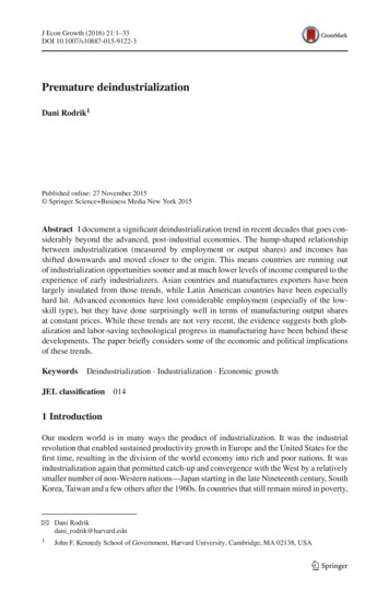
J Econ Growth (2016) .81010.210.410.610.81111.211.411.611.8120Fig. 1 Simulated manufacturing shares as a function of income (In GDP per capital in 1990 internationaldollars)data indicate a much earlier decline, at less than half the pre-1990 income level. (Note thatthe peak shares themselves are less meaningful in the case of output, as they depend on thebase year selected for converting current prices to constant prices.)The literature focuses on two possible explanations for why manufacturing’s share eventually falls (Ngai and Pissarides 2004; Buera and Joseph 2009; Foellmi and Zweimuller 2008;Lawrence and Edwards 2013; Nickell et al. 2008). One is demand-based, and relies on a shiftin consumption preferences away from goods and towards services. This on its own wouldnot produce the timing difference in peaks, as a pure demand shift would have similar effectson manufacturing quantities (output and employment). The second explanation is technological, and relies on more rapid productivity growth in manufacturing than in the rest of theeconomy. As long as the elasticity of substitution is less than one, this produces a declinein the share of manufacturing employment, but not in the share of manufacturing output.We need a combination of supply- and demand-side reasons to explain both the decline inmanufacturing’s share and the later turnaround in output compared to employment.An added complication is that the effects of technology and demand shocks depend crucially on whether the economy is open to trade or not (Matsuyama 2009). For the moment, Ileave these questions aside. I will develop the analytical results linking technology, demand,and trade to deindustrialization in Sect. 7.As Fig. 1 shows, nommva also peaks much earlier than realmva, though not so early asmanemp. The explanation for this difference has to do with relative price changes over thecourse of development. The relative price of manufacturing tends to decline as countries getricher, tending to depress the share of MVA at current prices. Figure 2 displays the pattern forfour of the countries in our sample. The relative price of manufacturing has more than halvedin the United States since the early 1960s. Great Britain has experienced a somewhat smallerdecline. In South Korea, which has grown extremely rapidly, manufacturing’s relative price123
123 0.011 (0.006) 0.021 (0.007) 0.033 (0.008) 0.052 (0.009) 0.085 (0.010) 0.029 (0.005) 0.044 (0.006) 0.066 (0.007) 0.086 (0.009) 0.117 (0.010)Yes4219952000s Country fixed effectsNumber of countriesNumber of observations199542Robust standard errors are reported in parenthesesLevels of statistitical signficance: 99 %; 95 %; 90 %1990s1980s1970s1960sln GDP per capita squaredYes0.230 (0.031) 0.013 (0.002)0.321 (0.027) 0.018 (0.002)ln GDP per capita0.005 (0.001)199542Yes 0.035 (0.009) 0.011 (0.007) 0.017 (0.008) 0.004 (0.006) 0.008 (0.005)0.204 (0.025) 0.009 (0.001) 0.113 (0.028)0.142 (0.029) 0.002 (0.001)0.115 (0.021) 0.000 (0.001)ln population squared220942Yes 0.105 (0.009) 0.054 (0.006) 0.074 (0.008) 0.018 (0.004) 0.033 (0.005)0.316 (0.026) 0.018 (0.002) 0.001 (0.001)0.122 (0.021)manemprealmvamanempnommvaLargest sampleCommon sampleln populationTable 2 Baseline regressions212842Yes 0.085 (0.010) 0.028 (0.008) 0.049 (0.009) 0.010 (0.006) 0.014 (0.007)0.266 (0.031) 0.014 (0.002) 0.004 (0.001)0.192 (0.027)nommva230242Yes 0.059 (0.011) 0.040 (0.010) 0.034 (0.009) 0.026 (0.008) 0.028 (0.007) 0.012 (0.002)0.262 (0.027)0.003 (0.001) 0.039 (0.025)realmva8J Econ Growth (2016) 21:1–33
23491relative price deflator of manufacturingJ Econ Growth (2016) ig. 2 Relative price trendshas come down by a whopping 250 %. In Mexico, meanwhile, relative prices have remainedmore or less flat.These trends are also consistent broadly with a technology-based explanation for themanufacturing hump. More rapid productivity growth in manufacturing reduces the relativeprice of manufactured goods through standard supply-demand channels. This in turn causesnommva to reach an earlier peak than realmva as shown in Fig. 1.3 Deindustrialization over timeAs Fig. 1 makes clear, deindustrialization is the common fate of countries that are growing.My interest here is to check whether deindustrialization has been more rapid in recent periods.For this purpose, I use a basic specification that controls for the effect of demographic andincome trends (with quadratic terms for log population, pop, and GDP per capita, y) as wellas country fixed effects (Di ). The baseline regression looks as follows:manshar eit β0 β1 ln popit β2 (ln popit )2 β3 ln yit β4 (ln yit )2 γi Di ϕT P E RT it ,iTwhere manshar e denotes one of our three indicators of industrialization. Country fixedeffects allow me to take into account any country-specific features (geography, endowments,history) that create a difference in the baseline conditions for manufacturing industry acrossdifferent nations. My main focus is on trends over time, which are captured using perioddummies (P E RT ) for the 1960s, 1970s, 1980s, 1990s, and post-2000 years. (The post-2000dummy covers the period 2000 through the final year in the sample, 2012.) The estimatedcoefficients on these dummies (ϕT ) allow us to gauge the effects of common shocks felt bymanufacturing in each of the time periods, relative to the excluded, pre-1960 years.Table 2 shows two versions of the baseline results for each of our three measures ofmanufacturing industry, manemp, nommva, and reamva. Columns (1)–(3) are restricted to acommon sample so that the results are directly comparable across the measures. Columns123
10J Econ Growth (2016) 21:1–33(4)–(6) employ the largest sample possible. The common samples have 1995 observations,while the others range from 2128 to 2302.The results for manemp and nonmva are very similar across the two specifications. Inboth cases, we find a sizable and significant negative trend over time, larger for manempthan for nonmva. Using the estimates from the common sample, the average country in oursample had a level of manemp that stood 11.7 percentage points lower after 2000 than in the1950s, and 8.8 percentage points (0.117–0.029) lower than in the 1960s. The correspondingreductions for nommva are 8.5 and 7.4 % points, respectively.The declines in realmva are smaller, and in the common sample show up significantlyonly for the post-1990 period. Depending on whether we use the common or largest sample,the post-2000 negative shock is 3.5–5.9 % points relative to the pre-1960 period.Figure 3a–c provide a visual sense of the results. They plot the estimated coefficientsfor the period dummies, along with a 95 % confidence interval around them. The figuresshow a steady decrease over time in manufacturing shares after controlling for income anddemographic trends. The decline is most dramatic for employment; it is less pronounced,but still evident after 1990 for real MVA. Manufacturing employment and activity have gonemissing in a big way.The samples in Table 2 provide good coverage across developed and developing regions,but the number of countries is limited to 42. To make sure that the results are representativeof trends in other countries as well, I turn to the ADB dataset which includes a much largergroup of countries (up to 87 for manemp and 124 for nommva and realmva). The limitationin this case is that coverage begins in 1970 (Felipe and Rhee 2014). So I include dummiesfor the 1980s, 1990s, and post-2000 years only, with the 1970s as the excluded period. Notethat the ADB data set provides two alternative series for MVA, one using U.N. sources andthe other using World Bank data. The results are presented in Table 3, and are quite similarto the previous ones.Once again, the strongest downward trend over time is for manemp, a reduction of 6.5 %points compared to the 1970s. (This matches up well with the corresponding number of 7.3% points (0.117–0.044) from Table 2.) The decline in nommva is 3.0 or 5.2 points over the1970s, depending on which series is used. Finally, the decline for realmva is 0.9–2.4 points.4 Deindustrialization in differenty country groupsWe can obtain some insight about the causes of these trends by looking at deindustrialization patterns in different country groups separately. This is done in Tables 4, 5, and 6, formanemp, nommva, and realmva, respectively. In each table, the baseline regression is runfor the following groups: (a) developed countries; (b) Latin American countries; (c) Asiancountries; (d) sub-Saharan African countries; and (e) sub-Saharan African countries excluding Mauritius. Note that since there are no data for the 1950s for sub-Saharan Africa, theperiod dummies for that region start from the 1970s. Also, two of the countries our globalsample (Egypt and Morocco) do not belong in any of these groups, so have been excludedfrom the group-level estimations.99 An alternative, and more efficient form of estimation would be to introduce periodXgroup dummies in asingle, global regression. However, the results in Tables 4-6 suggest considerable heterogeneity in the estimatedcoefficients on population and income terms across groups. So allowing these coefficients to vary seems worththe price of potentially reduced power. Since the period dummies in the group-specific regressions are estimatedtightly for the most part, the loss in efficiency does not appear to make much practical difference.123
J Econ Growth (2016) 21:1–3311(a)01960s1970s1980s1990s2000 1960s1970s1980s1990s2000 1970s1980s1990s2000 8-0.1-0.12-0.14Fig. 3 Estimated period coefficients (with 95 % confidence intervals): a manemp b nommva c realmva123
123 0.029 (0.002) 0.052 (0.003) 0.043 (0.004) 0.065 (0.005)Yes8719471990s2000s Country fixed effectsNumber of countriesNumber of observationsRobust standard errors are reported in parenthesesLevels of statistitical signficance: 99 %; 95 %; 90 % 0.011 (0.002)4378124Yes 0.013 (0.001)0.238 (0.016)0.693 (0.052)ln GDP per capita 0.039 (0.003) 0.004 (0.001) 0.004 (0.001)ln population squared 0.023 (0.002)0.194 (0.026)0.196 (0.043)ln populationln GDP per capita squaredADB/UNADB/ILO1980snommvamanempTabl
5 This echoes the concern in the voluminous literature on the Dutch disease, that developing countries with comparative advantage in primary products would experience a squeeze on manufacturing as they open up to trade. See Corden (1984), van Wijnbergen (1984), and Sachs and Warner (1999). 123