Transcription
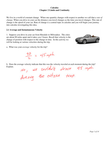
CalculusChapter 2 Limits and ContinuityWe live in a world of constant change. When one quantity changes with respect to another we call that a rate ofchange. When you drive in your car the distance you travel changes as the time you travel changes. This rate ofchange is the speed of your car. Rate of change is a central topic in calculus and you will begin your journeyinto calculus investigating this idea.2.1 Average and Instantaneous Velocity1. Suppose you drive in your car from Hinsdale to Milwaukee. The citiesare about 90 miles apart and it takes you 2 hours. Recall that velocity is thechange of position with respect to the change in time. In this activity wewill be looking at various velocities during the trip.a. What was your average velocity for the trip?b. Does the average velocity indicate that this was the velocity traveled at each moment during the trip?Explain.Page 1 of 14
CalculusChapter 2 Limits and ContinuityThe graph below is a plot of distance vs. time for your trip.Let’s call the function that pairs the distance traveled d in time t function f. So in function notation we haved f (t ) .c. Looking at the graph, describe this trip in words. That is, when were you speeding up, slowing down,stopped, and traveling at a constant velocity?d. From the graph find the values for f (0) and f (2) . Describe what these values mean in terms of your trip.Page 2 of 14
CalculusChapter 2 Limits and Continuitye. On the graph, connect the points 0, f (0) and 2, f (2) . Find the slope of this line. What does the slope ofthis line tell you about the trip?f. What was the average velocity during the second half of the trip where 1 t 2 ? Describe this averagevelocity in terms of slope.In general, the average rate of change for any function over any interval is the slope of the line joining theendpoints of that interval. This line connecting the endpoints is called the secant line. So we see that the slopeof the secant line represents the average rate of change.Page 3 of 14
CalculusChapter 2 Limits and Continuity2. Clearly you were not traveling at 45 mph throughout the entire trip. At some point you might be traveling 30mph or 75 mph or 0 mph. Your car’s speedometer indicates the instantaneous velocity at each moment in time.a. Suppose you want to know how fast you were traveling at exactly 1 hour 13 minutes and 28 seconds intoyour trip. How does calculating this instantaneous velocity pose a problem for us?Page 4 of 14
CalculusChapter 2 Limits and Continuityb. As you have discussed in the part a calculating the instantaneous velocity is not as simple as calculating theaverage velocity. So let’s think of some strategies for estimating the instantaneous velocity of our car at somemoment in time say t 1 hour into the trip. We will start with a graphical approach to this problem by zoomingin on the graph around the 1 hour mark as shown below.Page 5 of 14
CalculusChapter 2 Limits and ContinuityZooming in we get the following portion of the curve.The table below gives distance values for our trip at time values 0.25 hours before and after 1 hour.Pointtime (hr)distance (miles)B0.7525A1.0040.00C1.2546Remember that we want to determine our instantaneous velocity at the target point A. Since slopes of secantlines are easy to find and represent average rates of changes perhaps then we can use the slopes of secant linesto estimate the instantaneous rate of change. Draw a secant line connecting points A and B and another secantline connecting points A and C. Extend both of these secant lines through the graph. Calculate the slopes ofthese two secant lines.What do these slope values represent?Page 6 of 14
CalculusChapter 2 Limits and Continuityc. Do you think that either slope value is an accurate estimate for the instantaneous velocity at A? Explain.d. Sketch a line in the graph through the target point A whose slope you believe represents the instantaneousvelocity at A. What type of line does this line appear to be?e. Estimate the coordinates for a second point on the tangent line that you drew in part d and then using thetarget point at A calculate the slope of this line. Interpret this value in the context of this problem.Page 7 of 14
CalculusChapter 2 Limits and Continuity3. From the previous question we now know that the instantaneous velocity is graphically the slope of thetangent line at the target point 1, 40 . Let’s practice this strategy on our original graph for our trip toMilwaukee.a. On the graph below, use a ruler to draw a tangent line to the curve at 1 hours. Look along this tangent linefor another point on the line that is close to or right on the intersection of a pair of grid lines on the graph. Writethe coordinates of this point.b. Using the coordinates of the target point and the other point on your tangent line, calculate the slope of yourtangent line. Compare this value with others in your group. Interpret this value in the context of this problem.c. Find an equation for your tangent line (use point-slope form).d. Using a similar method, estimate the instantaneous velocity at 1.75 hours into the tripPage 8 of 14
CalculusChapter 2 Limits and Continuitye. Estimate when the instantaneous velocity of our car was the same as the average velocity for the entire trip.Discuss how you can find these values graphically.4. Suppose a tennis ball is dropped from a tall building and d the number of feet it falls in t seconds. Thefollowing table shows some of the values for distance and time.t (sec)d (meters)00115258312742025333a. Plot these six data points and connect them with a smooth curve. Appropriate label the axis and indicate theunits used.b. Calculate the slope of the secant line from 1,15 to 4, 202 and interpret its meaning.Page 9 of 14
CalculusChapter 2 Limits and Continuityc. Suppose we want to calculate the instantaneous velocity of the ball at t 2 seconds. Graphically what arewe interested in finding?d. You should realize from part c that we need to estimate the slope of thetangent line at 2 seconds. We could carefully draw the tangent line at 2 secondsand then try to estimate a second point on that tangent line to calculate the slope.We did this in the previous problem to estimate our instantaneous velocity at 1hour and 1.75 hours. However, since we have a table of values for the positionof the ball at various times we will make use of these table values and use adifferent strategy for estimating the slope of the tangent line. Let’s make threeestimates for the instantaneous velocity of the ball at t 2 seconds. by findingthe slope of the secant lines for the following (in each case carefully sketch thecorresponding secant line using a straight edge):i. from t 1 to t 2ii. from t 2 to t 3iii. from t 1 to t 3e. Of the three estimates from part d which do you believe is the best estimate for the velocity of the ball att 2 seconds? Explain your reasoning graphically.Page 10 of 14
CalculusChapter 2 Limits and ContinuitySo we have seen that one possible strategy for finding the slope of the tangent line is to simply draw the tangentline to the curve at the target point and estimate a second point on this line. Then use this point together with thetarget point to calculate the slope. This is a reasonable graphical approach however, as you have probablynoticed, we find that it’s not very accurate since it depends on how each of us draws the tangent line and on ourestimates for points on this line. We have also seen that another possible strategy is to pick two known pointson the curve that when connected produce a secant line that “looks” parallel to the tangent line our target point.We then use the slope of this secant to estimate the slope of the tangent line since lines that are parallel have thesame slope. You might have also averaged the slopes of secant lines connecting points on either side of thetarget point with the target point as an estimate for the slope of the tangent line. These are all valid graphicalstrategies but they don’t seem to be very mathematical and depend too much on estimates. Clearly we need amore mathematical strategy.Page 11 of 14
CalculusChapter 2 Limits and Continuity5. Let’s return to the graph below for our trip to Milwaukee and lets investigate a more mathematical strategyfor finding the instantaneous rate of change (slope of the tangent line) at 1 hour into our trip.a. We have already seen that the slopes of the secant lines AB and AC are not good estimates for the slope ofthe tangent line at point A. But maybe we can improve these estimates.Let’s consider the secant line AB . Draw that secant line above and discuss how you might move point B sothat the slope of this secant line is a better estimate for the slope of the tangent line at A.Page 12 of 14
CalculusChapter 2 Limits and Continuityb. Open the Sketchpad file HCtoMilwaukee. Display the secant line AB by clicking the button. Now grab point B and move it closer to point A. Describe what appears to behappening to this secant line.c. . What is a good estimate for the instantaneous velocity at 1 hour into our trip?d. Click the button. What is the slope of the tangent line? How good was yourestimate from part c? How close is the secant line to this tangent line?e. As you have seen in this activity, if we move point B “really close” to point A we see that the secant linebecomes nearly coincident to the tangent line and that the slope of the secant line is nearly equal to the slope ofthe tangent line. So the big question now is how close is “really close” and when is it close enough? Discussthis idea.Page 13 of 14
CalculusChapter 2 Limits and ContinuityNotesPage 14 of 14
2. Clearly you were not traveling at 45 mph throughout the entire trip. At some point you might be traveling 30 mph or 75 mph or 0 mph. Your car's speedometer indicates the instantaneous velocity at each moment in time. a. Suppose you want to know how fast you were traveling at exactly 1 hour 13 minutes and 28 seconds into your trip.