Transcription
Modeling Parabolic TroughSystemsSAM WebinarMike WagnerJune 18, 2014 1:00 p.m. MDTNREL is a national laboratory of the U.S. Department of Energy, Office of Energy Efficiency and Renewable Energy, operated by the Alliance for Sustainable Energy, LLC.
SAM Webinar Schedule for 2014ScheduleDetails New Features in SAM 2013 andBeyond oOctober 9, 2013: Paul GilmanoDecember 11, 2013: Janine FreemanoFebruary 12, 2014: Janine FreemanoApril 16, 2014: Paul GilmanoJune 18, 2014: Michael WagneroAugust 27, 2014: Aron DobosSAM PV Model Validation usingMeasured Performance DataSolar Resource Data 101Analysis of Electricity Rate Structuresfor Residential and CommercialProjects SAM 2014.1.14All sessions last one hour and beginat 1 p.m. Mountain TimeYou must register to participateRegistration is free, but space islimitedMore details, registrationinformation, and recordings of pastwebinars on Learning page of SAMwebsiteModeling Parabolic Trough SystemsPhotovoltaic Shading rning-sam2
OutlineSAM 2014.1.14 Overview of SAM Parabolic Trough Models Case study:Molten Salt Trough w/ Dry CoolingooooooHTF selectionModifying operating temperaturesLoop configuration and sizingPower cycle design point specificationOptimization of design parametersOptimization of TES and Solar Multiple3
This webinar is most useful if you have SAM 2014.1.14 Familiarity with parabolic trough technologycomponents and configurations A basic understanding of thermodynamics,heat transfer, and fluid mechanics Some experience using SAM Particular interest in technology(vs. cost/financial)4
Parabolic Trough TechnologySAM 2014.1.145
SAM Trough Performance ModelsSAM 2014.1.14 PhysicalooUses first-principle and semi-empirical models to calculateperformanceAllows modification of geometrical and optical propertiesto predict performance in new design spacesToday’s webinar uses the Physical Trough model EmpiricaloooPerformance based on empirical correlations from SEGSplant dataMost accurate for SEGS-like configurations, temperatures,& sizesMuch less computationally expensive than Physical model6
Physical Trough sub-modelsSAM 2014.1.14Collector and ReceiverOptical gain & thermal lossHTF distributionand transportPower CycleSteam generationTurbine & feed-waterHeat rejectionFossil backupThermal StorageStorage tanksHeat exchanger (indirect)7
Inputs in SAMSAM 2014.1.14The performance model input pages are where youdefine the system’s design parametersThe Costs, Financing and Incentives pagesdetermine the renewable energy system’s cost ( )8
SAM Trough DemoMolten Salt Trough with Dry Cooling9
What’s interesting about molten salt? SAM 2014.1.14Higher operating temperature than oil HTF’sGain in power cycle conversion efficiencyLower cost than oilMore energy-dense thermal storage“Direct” thermal storageSubstantially different thermal propertiesHigher freezing temperatureHigher thermal lossMore corrosive10
Analysis questionsSAM 2014.1.14 How much economic benefit can a moltensalt-based trough provide? What are the system-level design issues for aMS trough? What thermal storage size is most costeffective?11
The modeling process in SAM1.2.3.4.5.6.7.8.9.SAM 2014.1.14Configure receiver and collector componentsSpecify HTF and operating temperaturesDetermine transport operation limitsConfigure the loopSpecify power cycle design pointSpecify thermal storage parametersUpdate costs and financialsOptimize uncertain parametersOptimize solar multiple and TES capacity12
Receivers and CollectorsSAM 2014.1.14 Receivers (HCEs)oLoop thermal efficiency calculation uses the receiverEstimated avg. heat loss, which must be supplied bythe user.Annulus gas type (1) AiroEstimated average heat loss [310, 590, 4518,0]o– We are modeling molten salt, so hydrogen permeation is nota problem.– These values can be calculated based on detailed collectorperformance models, or by running the model andinspecting the results near design-point conditions Collectors (SCAs)oConfiguration name Solargenix SGX-113
Heat Transfer Fluid DifferencesSAM 2014.1.14Nitrate SaltTherminol VP1HitecNitrate SaltTherminol VP1HitecDowtherm QDowtherm RPDowtherm ADowtherm QDowtherm RPDowtherm A0.0125000.0082000Density (kg/m 3)Viscosity (Pa-s) Viscosity, density, and heat capacity differ substantially Pressure loss higher in salt system at equivalent 500Temperature (C)60070000100200300400500600Temperature (C)14700
Solar field – Min/Max Flow RateSAM 2014.1.14 Field HTF Fluid Hitec solar salt Design loop outlet temp 550 CoField inlet temperature related to boiling saturationtemperature Min/Max single loop flow rateooooPrimary concern is maximum pressure dropTherminol VP-1 velocity range [0.36, 4.97 m/s]Method (1): Manually try different loop lengths and flowrates in SAMMethod (2): Match pressure drops by iteratively solvingpipe pressure loss equations 15
Calculating pressure loss in a pipeSAM 2014.1.1416
(1) Establish a reference pressure loss Use Therminol-VP1 settings to calculate areference pressure lossoUse maximum Therminol velocityoCalculate Reynolds numberoLook up friction factor on Moody ChartoInitial reference length is 𝑙𝑟𝑟𝑟 1.0oSolve pressure loss eqn. for Δ𝑃𝑟𝑟𝑟 We will try to set up the salt loopto match this ref. pressure constantSAM 2014.1.14𝐷 0.066 𝑚𝑚𝑉𝑇 5𝑠𝑅𝑒𝑇 𝜌𝑇 𝑉𝑇 𝐷 1.39e6𝜇𝑇𝑓𝑓𝑓 0.011Δ𝑃𝑟𝑟𝑟𝜌𝑇 𝑉𝑇2 𝑙𝑟𝑟𝑟 𝑓𝑓𝑓 𝑅𝑒𝑇2𝐷 1610 𝑃𝑃17
(2) Calculate salt mass flow rate Use energy balance tocalculate mass flow rateooAbsorption energy balanceFirst-law balance Need to guess number ofSCA’s!o(will refine with iteration)SAM 2014.1.14𝑞̇ 𝑙𝑙𝑙𝑙 𝐴𝑠𝑠𝑠 𝜂𝑎𝑎𝑎 𝑁𝑠𝑠𝑠 𝐼𝑏𝑏𝑞̇ 𝑙𝑙𝑙𝑙 𝑚̇𝑠 𝑐𝑝𝑝 Δ𝑇𝑠𝑚̇𝑠 𝐼𝑏𝑏 950𝐴𝑠𝑠𝑠 𝜂𝑎𝑎𝑎 𝑁𝑠𝑠𝑠 𝐼𝑏𝑏𝑐𝑝𝑝 Δ𝑇𝑠𝑘𝑘 6.4𝑠𝑊𝑚2𝑐𝑝𝑝 1520𝐽𝑘𝑘 𝐾𝐴𝑠𝑠𝑠 470.3 𝑚2𝜂𝑎𝑎𝑎 0.689Δ𝑇𝑠 550 293 257 𝐶18
(3) Calculate velocity and new length Calculate velocity for mass flow rate Calculate Reynolds number Look up friction factor Solve pressure eqn. for length The new length is used to update theestimate of No. of SCA’soPressure highly nonlinear! Be conservative 𝑉𝑠 𝑅𝑒𝑠 𝑚̇𝑠𝐷𝜌𝑠 𝜋22SAM 2014.1.14𝑚 1.02𝑠𝜌𝑠 𝑉𝑠 𝐷 75254𝜇𝑠𝑓 𝑅𝑒𝑠 0.0195′𝑙𝑟𝑟𝑟 Δ𝑃𝑟𝑟𝑟 2𝐷 5.75𝜌𝑠 𝑉𝑠2 𝑓𝑓𝑓′𝑁𝑠𝑠𝑠 46?′′ 2 𝑁𝑠𝑠𝑠 16𝑙𝑟𝑟𝑟19
(4) Finally. Iterate to convergence on LIter1𝒎̇𝒔kg/s𝑽𝒔m/s𝑹𝒆𝒔SAM 𝒇 814311.21.801328020.0172.1116 Number of SCA/HCE Assemblies 14 Max HTF Flow rate 12.8 kg/s Min HTF Flow rate 1.75 kg/s20
Other Solar Field SettingsSAM 2014.1.14 Min/Max Header Velocity [0.7 m/s, 1.2 m/s] Freeze protection temp 260 CoMust maintain HTF above freezing temperatureoRelatively large field, so increase divisions. Ultimately, aparametric simulation can be run to determine which layout isbest Number of field subsections 8PPA price14.814.7514.714.6514.614.5514.5246810Number of Field Subsections1221
Power Cycle – Dry CoolingSAM 2014.1.14 Condenser type Air-cooled Ambient temp at design 42 CoCondensing temperature is 𝑇𝑎𝑎𝑎 Δ𝑇𝐼𝐼𝐼 58𝐶 Rated cycle conversion efficiencyPrefer detailed external model, but not always availableReference cycle – Molten Salt power tower w/ 550 C steamtemperature at 41.2% gross efficiencyo Assume 20 C salt-to-steam temperature dropo When in doubt, use Carnot scaling:oo58 273.15 0.5977𝟓𝟓𝟓 273.1558 273.15𝜂2 1 0.5877𝟓𝟓𝟓 273.15𝜂𝜂 0.412 𝜂2 0.40511– 𝜂1 1 ––22
Power cycle – Other parametersSAM 2014.1.14 Design gross output 167 MWeoIncrease design gross until the estimated nameplatecapacity meets the target Aux heater outlet set temp 550 CoNot used in this example, but good practiceoTrade HTF temperature for lower-efficiency cycle operationOptimize! Minimum required startup temp 360 Co23
Thermal storage parametersoEnsure HTF Hitec Solar SaltoTank height 15SAM 2014.1.14– No intermediate HX is required– How reasonable is the calculated tank diameter?Parallel tank pairs 2o Cold tank heater set point 260 Co– Match freeze protection temperature settingoHot tank heater set point 525 C– Don’t allow significant decay in hot TES temperature24
CostsSAM 2014.1.14 This example doesn’t consider detailed costinformation!oMinor changes to reflect updated HTF Storage cost 30 /kWht Power plant 1200 /kWe25
Simulation & Results (in SAM)26
Optimizing thermal storage and solar multipleSAM 2014.1.1427
Optimizing SAM 2014.1.1428
Comparison: MS vs Oil troughMS OptimizedMetricAnnual EnergyPPA priceLCOE NominalLCOE RealInternal rate of return (%)Minimum DSCRNet present value ( )Calculated ppa escalation (%)Calculated debt fraction (%)Capacity factorGross to Net Conv. FactorAnnual Water UsageTotal Land AreaValue746,036,992 kWh14.16 /kWh16.80 /kWh13.58 /kWh19.35%1.43 137,266,240.001.00%50.00%56.70%0.93141,351 m31961.13 acresOil Trough OptimizedMetricAnnual EnergyPPA priceLCOE NominalLCOE RealInternal rate of return (%)Minimum DSCRNet present value ( )Calculated ppa escalation (%)Calculated debt fraction (%)Capacity factorGross to Net Conv. FactorAnnual Water UsageTotal Land AreaSAM 2014.1.14Value349,266,368 kWh15.30 /kWh19.24 /kWh15.55 /kWh19.50%1.44 73,059,680.001.00%50.00%39.90%0.931,317,661 m3898.08 acres29
18.06.2014 · Therminol VP-1 velocity range [0.36, 4.97 m/s] o. Method (1): Manually try different loop lengths and flow rates in SAM . o. Method (2): Match pressure drops by iteratively solving pipe pressure loss equations 16 . SAM 2014.1.14 . Calculating pressure loss in a pipe . 17 SAM 2014.1.14 (1) Establish a reference pressure loss Use Therminol-VP1 settings to calculate a reference pressure .