WIXLIB

Donor Segmentation and Analysis Using Microsoft Excel Pivot TablesIntroductionDonor database segmentation and analysis expose important trends and focuses our attentionon our best prospects. This how-to session focuses on the most powerful and underutilizedfeature of Microsoft Excel – the Pivot Table – for performing simple do-it-yourself databasesegmentation. Pivot tables transform up to one million rows of data into multiple summarycharts and graphs in mere seconds. No other tool in Excel gives you this flexibility andanalytical power. You will walk away with powerful sample charts that you or an Excelsavvy colleague can create when you get back to the office.This paper first describes why you might want to use pivot tables. Second, the paperdiscusses resources and tutorials available to help you understand the fundamentals of pivottables. A discussion follows on data requirements. And finally, seven sample pivot tablesare presented. These samples may be used as a “recipe” to create pivot tables with your owndata.While not illustrated here, the reader should note that pivot tables have a powerful drilldownfeature so you can see the data behind the pivot table numbers. To activate this featuredouble click on any pivot table cell. For example, assume you created a simple pivot tablethat in part reveals the following information: 35 donors gave 5,000 or more in the year2008. Simply double click on the number 35 and a list of those 35 donors will appear in anew window. Don’t worry if this explanation is not completely clear at this point. Just giveit a try after you create your first pivot table and the benefits will become obvious!Why Use Pivot Tables?Seven key reasons for organizing your donor data into pivot tables are to:1.2.3.4.5.6.7.summarize large amounts of donor data in a meaningful waycreate multiple unique perspectives of your datafind relationships and groupings within your datacreate a list of unique values for one field in your dataexpose trends for various time periodsaccount for frequent requests for updates to analysisorganize data into format that is easy to convert into a chartResourcesWith a little bit of practice, creating pivot tables is not difficult. Documentation -- bothonline tutorials and in book format-- is abundant and readily available so detailed instructionson the basics will not be repeated here. One book provided me with all of the information Ineeded to master the basics. The title is Pivot Table Data Crunching for Microsoft OfficeHodes1

Excel 2007. It is written by Bill “Mr. Excel” Jelen and Michael Alexander. As ofpublication it was available used on Amazon for 17.29. All of the basics appear in chapter1 through 4 and chapter 6. Alternatively, the reader may do a Google search on “PivotTables” and find a variety of online tutorials free of charge.Data PreparationThe data used to create the seven pivot tables presented in this paper was exported fromRaiser’s Edge (RE). As long as the database you use has the ability to export its data into afile importable into Microsoft Excel, you will be able to create pivot tables. In RE, exportthe following fields to perform the data analysis: (1) first gift date; (2) last gift date; (3) total# of gifts; (4) total dollar amount given; (5) amount given by calendar year (e.g., 2006, 2007,2008, 2009, and 2010);In addition, export the following fields for reference purposes: (1) Contact information suchas name, spouse name, phone number, address (city, state, and zip as separate fields); (2)purchased screened information (e.g., age, wealth indicators, income) and (8) internallycreated fields (e.g., donor id, membership in bequest society, assigned solicitor).Appendix A is an instruction sheet you can modify to suit your needs and share with yourdatabase administrator.Your pivot table experience will be greatly enhanced by starting with a well prepared datafile. Adhere to the following guidelines and you should not have any problems (see Figure 1as an example):1. Remove blank rows or columns2. Every column must have a brief heading. Replace the very long column headings thattypically appear on a Raiser’s Edge export with brief descriptors (e.g., Total #, TotalAmt)3. Ensure that every numerical cell has a value (refer to the bottom of page 25 of PivotTable Data Crunching for Instructions). Blank cells should be replaced with a zero.Figure 1.Sample Data LayoutHodes2

Sample Pivot TablesThis section contains seven sample pivot tables that you can create using your own data.Each sample includes a description, a picture of the pivot table, a list of data fields required,and step by step instructions for pivot table creation. These are simply samples to get youstarted. The pivot tables you decide to create are only limited by the data available to youand your creativity and imagination.Sample Pivot Tables:1. Recency, Frequency2. Recency, Frequency, Monetary3. Cumulative Amount Given Pivot Table with Pivot Graph4. Giving Level for Year 20095. Giving Level for Year 2009 for New Donors Only6. Donor Acquisition and Retention7. Change in Giving 2009 versus 2008Hodes3

Sample 1: Recency, Frequency, (RF) Pivot TableDescriptionRFM (Recency, Frequency, Monetary) analysis is a marketing technique used to determinequantitatively which donors are “the best ones” by examining how recently a donor made agift (recency), how many times they have made a gift (frequency), and amount donated(monetary). The idea underlying RFM analysis is that donors who have given recently, havea larger total number of gifts, and have made larger gifts, are likely our best prospects forfuture large gifts. Alternatively, RFM analysis could be used to target planned givingmessages to lapsed donors who have made a large number of gifts, or to urge donors whohave made fewer and smaller gifts to renew at a higher level. RFM analysis is not a panaceabut has the advantage of using information about a donor’s past behavior that is easilytracked and readily available in your donor database.We begin by first examining the two dimensional Recency – Frequency (RF) Pivot Table inthis section and then advance to the three dimensional RFM Pivot Table in sample 2.The pivot table in Figure 2 plots 13,332 donors by the last gift year (recency) and cumulativenumber of gifts (frequency). By way of example, focus your attention on the upper righthand corner of the chart. 1,873 donors made their last gift some time in 2010. Of thatamount, 56 of the donors have a cumulative number of gifts of 26 or greater.Figure 2.Sample Recency – Frequency Pivot Table–Sample 1 continued on next page.–Hodes4

Sample 1 (continued)Data Fields Required1. Last gift date2. Total number of giftsStep by Step Instructions (See Figures 2a and 2b for screenshots of some of these steps.)1. In the pivot table field list drag the field “total number of gifts” into the Column Labelssection. Group Starting at: 1, Ending at: 25, By: 5. Donors with more than 25 gifts willbe grouped into the category 26 gifts.2. Drag “last gift date” into the Row Labels section. Group Starting at: 1/1/2006, Ending at:12/31/2010, by: Year3. Drag “total number of gifts” into the Values Section. Set the Values Field Setting toCount.Hodes5

Figure 2a.Figure 2b.Screenshot – The Group FunctionScreenshot – Setting Field Values to CountHodes6

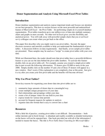
Sample 2: Recency, Frequency, Monetary (RFM) Pivot TableDescriptionFigure 3 adds the dimension of monetary contributions to sample 1. Observe that the same1,873 donors made gifts in 2010 (refer back to sample 1) and 56 of those donors havecumulative number of gifts of 26 or greater. But in addition you can see that 9 of the 56donors have a total dollar amount given somewhere between 1 and 1,000, 8 of the 56between 1,001 and 2,000, and 39 have total dollar amount given of greater than 2,000. Ifyou’ve already created the pivot table in sample 1, simply add to what you’ve already doneand proceed directly to step 4 below.And as I explained in the introduction, if, for example, you clicked on the cell containing the39 donors who gave over 2,000, Excel will create a”drilldown” list consisting of thesespecific donors.Figure 3.Sample Recency, Frequency, Monetary Pivot Table–Sample 2 continued on next page.–Hodes7

Sample 2 (continued)Data Fields Required1. Last gift date2. Total number of gifts3. Total dollar amount givenStep by Step Instructions1. In the pivot table field list drag the field “total number of gifts” into the Column Labelssection. Group Starting at: 1, Ending at: 25, By: 5. Donors with more than 25 gifts willbe grouped into the category 26 gifts.2. Drag “last gift date” into the Row Labels section. Group Starting at: 1/1/2006, Ending at:12/31/2010, by: Year3. Drag “total number of gifts” into the Values Section. Set the Values Field Setting toCount.4. Drag “total dollar amount given” into the Row Labels section. Group Starting at: 1,Ending at: 2,000, by 1,000.Hodes8

Sample 3: Cumulative Amount Given Pivot Table with Pivot GraphDescriptionFigure 4 is a count of the number of donors whose total cumulative amount given fits intoeach 500 band. This is the monetary contribution (M) component of the pivot table createdabove. This simple pivot chart and graph use only one piece of data – Total Amt. It givesthe user a very quick picture of the number of donors that fit into various giving categories.Note below that the overwhelming majority of donors (10,956) have a cumulative amountgiven of 500 or less. Only 409 donors have total giving over 3,000.Figure 4.Cumulative Amount Given Pivot Table with Pivot GraphData Fields Required1. Total dollar amount givenStep by Step Instructions1. Drag “total dollar amount given” into the Row Labels section. Group Starting at: 1,Ending at: 3,000, by: 500.2. Drag “total dollar amount given” into the Values Section. Set the values field setting toCount.3. On the main Excel ribbon Click Options – Pivot Chart in order to create the graph. SelectColumn as the type of graph. Go to the Layout section of the ribbon and you will havethe option of creating chart and axis titles, data table, etc. Play with the various menus tobecome familiar with options that are available.Hodes9

Sample 4: Giving Level for Year 2009 – Viewing the Same Data in Four Different WaysDescriptionAt first glance Figure 5 appears to be a complex chart requiring four fields of data. In factone piece of data –“amount given year 2009” is simply displayed in four different ways.This chart not only provides some very useful information but it also illustrates the power ofPivot Tables to create multiple unique perspectives of your data with the simple click of amouse.By way of example the chart is explained. There are 5,856 donors (of the total 6,185 donors)that gave a total amount in 2009 between 1 and 500. These 5,856 donors represent 94.7%of the number of donors, gave a cumulative total of 481,979 in gifts, and account for 27.6%of the total amount given.Figure 5.2009 Giving LevelsField Required1. Amount given in year 2009Step by Step Instructions1. Drag “amount given year 2009” into the Row Labels Section. Group Starting at: 1,Ending at: 2,000, by: 500.2. Drag “amount given year 2009” into the Values Section. Set values field setting toCount.3. Drag “amount given year 2009” into the Values Section. Set the values field setting to %of Count.4. Drag “amount given year 2009” into the Values Section. Set values field setting to Sum.5. Drag “amount given year 2009” into the Values Section. Set values field setting to % ofSum.Hodes10