WIXLIB

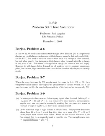
14.64:Problem Set Three SolutionsProfessor: Josh AngristTA: Amanda PallaisDecember 1, 2009Borjas, Problem 3-6In this set-up, we need an instrument that changes labor demand. (As in the previouschapter, we could also use an instrument that changes wages by at such as eligibilityfor the EITC. It’s hard to think of a factor that leads to a change in labor demand,but not labor supply. One instrument that changes labor demand might be a changein the price of oil. This doesn’t change labor supply (in terms of the real wage).However, it will change labor demand for oil workers, energy company employees,pilots, bus drivers, ‡ight attendants and other industries that rely disproportionatelyon oil.Borjas, Problem 3-7When the wage increases by 5%, employment decreases by 0:4 5% 2%: In acompetitive labor market, the wage is the productivity of the last worker. So, if thewage increases by 5%, the marginal productivity of the last worker increases by 5%.Borjas, Problem 3-9(a) In a competitive labor market, labor supply equals labor demand. Solving Es Ed gives E 16 and w 6. In a competitive labor market, unemploymentequals zero. not everyone is necessarily working, but everyone who wants towork at a wage of 6 gets to, so there is no unemployment.(b) If the minimum wage is eight dollars, it clearly binds. Employment demandeddrops from 16 to 8, so 8 people lose their jobs. At a wage of 8, E S 18 so 2more people want to work than before. There are ten workers who want a jobbut cannot nd it, so unemployment is equal to ten. The unemployment rateunemployed10 8 10 59 : employed unemployed1

Borjas, Problem 3-12The higher the elasticity of labor demand, the more labor demand decreases whenthe wage increases. thus, the minimum wage will lead to more unemployment whenthere is a high elasticity of labor demand. I would think that labor demand is moreelastic in the lawn-care industry than in the fast-food industry. When the price oflawn-care workers increases, consumers have more options that didn’t face the sameincrease in price. They can hire a neighbor who is not subject to the minimum wageto cut their grass, hire an illegal immigrant (many of whom work in these types ofindustries in the West) or do it themselves. Consumers in a fast food restaurant maynot be as elastic in their demand, so that the labor demanded for fast food workersmight not fall as much in response to an increase in wages. Thus, employment in theminimum wage would have a greater e ect in the lawn-care industry.Borjas, Problem 4-5(a) Remember that labor and wages are jointly determined by the monopsonistwithpf 0 (L) w(L)[1 ]:If there exists a payroll tax then we must replace w(L) withw(L), where 1 is some factor that adjusts for the fact that the monopsonist will have topay higher wages now. (Who bears all of the tax is a seperate question.) Thisleads to a lower equilibrium wage and employment overall. In the monopsonygraph we always stare at, this means that the w(L) curve shifts even fartherleft.In a perfectly competitive labor market, the demand curve will shift in as a resultof the tax, leading to lower wages and employment, as well. But remember thatthe competitive market had a higher level of employment to begin with.(b) A perfectly discriminating monopsonist is a monopsonist that can pay each ofhis workers a di erent wage. He will hire the perfectly competitive numberof workers, because the perfectly discriminating monopsonist does not have toworry about how the marginal worker’s wage a ects the wages of the inframarginal workers. Consequently, the minimum wage would lower employment (if itbinds) and raise average wages.Borjas, Problem 4-10(a) If Ann uses push mowers, each laborer will take two hours to cut each lawn. Soshe will have to demand 400 2 800 hours of labor. That’s a total labor costof 5 800 4000 dollars. Each worker can supply a total of 8 5 40 hoursof labor a week, so she would need 20 workers and 20 push mowers.2

(b) If Ann uses riding mowers, each laborer will take half an hour to cut each lawn.So she will have to demand 400 12 200 hours. Each worker can supply 40hours of labor, so she would only need ve laborers and ve riding mowers.That’s a total labor bill of 5 200 1000 dollars.(c) We can compare total costs under the two technologies. Using push mowers,her total costs are 250 20 5 20 40 9000. Using riding mowers, hertotal costs are 1800 5 5 5 40 10000. So she’ll use the less e cienttechnology, push mowers.(d) The costs for the push mowers are now (250(1 0:2)) 20 (5(1 0:2)) 40 20 8800. The costs for riding mowers are now (1800(1 0:2)) 5 (5(1 0:2))20 40 8400. So Ann will now switch to the more advanced technology.Borjas, Problem 6-1(a) If the interest rate is 5%, then in period 2 dollars Debbie earns15; 0001:05 472; 000 456; 250 as a marine biologist and40; 0001:05 500; 000 458; 000 as a concert pianist.So she will choose to be a concert pianist.If the interest rate is 15%, then in period 2 dollars Debbie earns15; 0001:15 472; 000 454; 750 as a marine biologist and40; 0001:15 500; 000 454; 000 as a concert pianist.So she will choose to be a marine biologist. The higher rate of interest meansthat from the standpoint of period 2 schooling costs incurred in period 1 becomemore expensive, so now the option with the lower schooling costs (and lowersalary) becomes more attractive.(b) Under this scenario in period 2 dollars, Debbie earns15; 0001:05 472; 000 456; 250 as a marine biologist and60; 0001:05 500; 000 437; 000 as a concert pianist.So she will choose to be a marine biologist.1Borjas, Problem 6-2If Peter avoids school the PDV of his lifetime earnings will be100 90110 1 0:2 (1 0:2)23254:

If Peter gets an undergraduate degree, this becomes50 180180 1 0:2 (1 0:2)2225:If Peter decides to go to graduate school, this becomes50 0 400(1 0:2)2227:It seems as though Peter should avoid education like the plague.Borjas, Problem 6-4If the rate of depreciation on human capital increases, then the PDV of future earningsgoes down. This provides less of an incentive to invest in human capital.Borjas, Problem 6-8For this to be an incentive compatible screening device, the low-ability workers shouldnot want to get the diploma. This means that their return from not getting thediploma (25 0) is greater than the return if they do get the diploma (K 20). Sowe must have K 20 25 or K 45. Additionally, the high-ability types must wantthe diploma, so K 8 25 0 or K 33. So we have 45 K 33.2B: Analytical Problem(a) The individual employer solvesmaxL f (L)wLmaxL ln(L)wLFOC:1L wSo an individual rm’s demand curve is L The agregrate demand curve is then L 1wNw(b) In a competitive market, labor demand equals labor supply:L Nw w"w" 1 Nwc N 1 (" 1)L N Lc Nw NN 1 (1 ") N " (1 ")4

(c) Now the employer knows that if he demands more labor he also changes thewage. He solvesmaxL N f (L)w(L)LNote that labor supplied satis es L w" so that w L1 " so this becomesmaxL N ln(L)L1 " LmaxL N ln(L)L(1 " ")N( 1 ")L1 "L"N ( 1 ")L1 "L""N ( 1 ") L(1 ") "FOC: 0" " (1 ")L N Lm N " (1 ") ( 1 ")" " (1 ") 1 ")]wm L1 " [N " (1 ") ( 1 "" 1 (1 ")wm N 1 (1 ") ( 1 ")(d) Note that in the perfectly competitive case, wc N 1 (" 1) ; whereas in the" 1 (1 ")): The only di erence is the factormonopsony case, wm N 1 (1 ") ( 1 "" 1 (1 ")( 1 " )in the monopsony case." 1 (1 ")) 1 and wages are always higher in the competitive case.Since " 0; ( 1 "Similarly, the only di erence between employment in the perfectly competitive" " (1 ")and monopsony case is that there is an extra factor of ( 1 ") 1 in themonopsony level of employment, leading the monopsony level of employment tobe lower than in the perfectly competitive case." 1 (1 ")" " (1 ")If ( 1 ") ( 1 ") 1; then wages and employment would be in thesame in the monopsony and perfectly competitive cases. If " 1; then bothof these equal one. So if the labor supply elasticity (") equals in nity or laborsupply is perfectly elastic, there is no di erence in these two cases.(e) It can set a minimum wage equal to the competitive wage. If it does this, thenit will bind. The monopolist will then choose the level of employment thatmaximizes his pro ts, which is the competitive level of employment.5

Problem C1. What is the net present value at the start of life of getting s years of schooling? From lecture: PDV (s) f (s)e rt dt sf (s) rser2. Assuming that market forces equalize the value of alternative schooling plans, derive anequation for lnf(s) in terms of lnf(0), r and s.PDV(S s) PDV(S 0), for all s. So:f (s) rsf (s). Taking logs of each side:e PDV (S 0) rrln( f (s)) rs ln( f (0)) ln( f (s)) ln( f (0)) rsPDV (S s) 3. How does a change in the interest rate, r, affect the relationship between schooling andearnings? Why?For a given level of schooling, a higher interest rate implies that earnings after schooling mustbe higher. This is because a higher interest rate means that benefits that accrue in the future areworth less to you today (if you think of r as an interest rate, this is because it is more expensiveto borrow against future earnings; if you think of r as a discount rate, this is because youdiscount future benefits more heavily). Since earnings from any amount of schooling must equalearnings from no schooling, a higher interest rate means that earnings for schooling must behigher than before in order for anyone to want to get schooling.4. Suppose that smart people, i.e. those with big earnings potential, get paid a subsidy foreach year they go to school. The subsidy is s*c*f(0) for someone who goes s years, where cis a constant between 0 and 1. The subsidy is paid up front when you start school.Assuming that market forces equate the NPV of schooling plans, derive an equation forlnf(s) in terms of lnf(0), r, s , and c. How does the subsidy affect the relationship betweenschooling and earnings? Why?f (s) rsf (0). Rearranging:e scf (0) rrln( f (s)) ln( f (0)) rs ln(1 scr)We’ll have to assume that c*r is low enough such that 1-scr 1, so that ln(1-scr) is defined.Assuming this, then ln(1-scr) 0, and so for a given level of schooling, the subsidy reduces theearnings that one receives after schooling. This is because the subsidy provides an additionalmonetary benefit for schooling (or, think of it as a reduction in schooling costs) – so for peopleto be indifferent between schooling and no schooling (which happens due to market forces, inthis model) the earnings for a given level of schooling must be lower under the subsidy caserelative to the no subsidy case.PDV (S s)

You could also note that the returns to schooling (i.e. the increase in “wage” for an increase incrschooling) decrease from r to r .1 scr