Transcription
Hierarchical Path Planner using Workspace Decompositionand Parallel Task-Space RRTsGeorge Mesesan1 , Máximo A. Roa1 , Esra Icer2 , and Matthias Althoff2Abstract— This paper presents a hierarchical path plannerconsisting of two stages: a global planner that uses workspaceinformation to create collision-free paths for the robot endeffector to follow, and multiple local planners running inparallel that verify the paths in the configuration space byexpanding a task-space rapidly-exploring random tree (RRT).We demonstrate the practicality of our approach by comparingit with state-of-the-art planners in several challenging pathplanning problems. While using a single tree, our planneroutperforms other single tree approaches in task-space orconfiguration space (C-space), while its performance and robustness are comparable or better than that of parallelizedbidirectional C-space planners.I. I NTRODUCTIONFinding a collision-free path for a robot is a decades-oldproblem in robotics. Solutions have been proposed usingmainly two approaches: sampling- and optimization-basedplanners. Sampling-based approaches work by randomlyproducing different robot configurations, verifying whichones are collision-free, and creating graph structures that canbe queried for a trajectory between the initial and final robotconfiguration. For static scenarios where multiple queries areperformed, probabilistic roadmaps (PRMs) [1] offer a goodsolution strategy. For single queries or non-static environments, rapidly-exploring random trees (RRTs) [2] have beenproposed. These techniques are probabilistically complete,but often require a post-processing step to smooth the resulting jerky trajectories. On the other hand, optimizationbased planners define a cost function to be minimizedwhile traveling from an initial to a goal configuration [3].These approaches suffer in general from problems such asnon-convergence or local minima, typically associated withoptimization methods. Also, on difficult path scenarios thatrequire more exploration than exploitation, these algorithmsmight fail to find the solution.Sampling-based path planners can search for a solutioneither in the configuration space (C-space) or in the taskspace. While C-space planners use a simplified representation of the robot as a point in a Rnq space, where nq isthe number of degrees of freedom (DoF) of the robot, thegoal also needs to be specified as a point (sometimes as aregion) in C-space. When a C-space goal point is directlyavailable, or can be easily computed, a bidirectional RRT*This work has received funding from the People Programme (MarieCurie Actions) of the European Union Seventh Framework ProgrammeFP7/2007- 2013/ under REA grant agreement number 608022.1 Institute of Robotics and Mechatronics, German Aerospace Center(DLR), 82234 Wessling, Germany. Contact: george.mesesan@dlr.de2 Department of Informatics, Technische Universität München, 85748Garching, Germanyapproach [4] is an efficient method of finding the solution.However, in many real-world path planning problems, a Cspace goal point is not available. As an example, considera redundant robotic manipulator whose task is to grasp anobject. The task may be specified simply as the position ofthe end-effector, which corresponds to an infinite number ofgoal configurations. Some of these configurations may not bereachable from the starting configuration of the robot, whileothers may lead to convoluted paths in configuration space.Based on these considerations, task-space approaches [5],[6] try to find a path for the robot by applying probabilistictechniques (like RRT) directly in the lower-dimensional taskspace Rnr (in the example mentioned above, nr 3). Atask-space tree can be grown using a Jacobian transpose[7] or a Jacobian pseudoinverse method [5]. An interestingbidirectional approach using both C-space and task-spacetrees was proposed in [8].A common method of improving the efficiency of pathplanning algorithms consists in using information extractedfrom the robot workspace. One approach used by C-spaceRRT planners is to bias the tree exploration using the obstaclegeometry [9], the medial axis of the free workspace [10],or spherical free-space regions computed on a generalizedVoronoi graph [11]. An alternative approach is to partitionthe free workspace into cells, and use their connectivity information. Tunnels of free workspace are constructed in [12] bya sphere expansion algorithm. An approximate cell decomposition of the workspace is used in [13] with a method fromimage processing called watershed segmentation to identifynarrow passages. Path planning problems involving roboticmanipulators typically have simpler workspace topologies,which make it possible to use exact cell decompositionsbased on convex shapes [14], intersecting convex shapes[15], or a combination of convex volumes and generalizedcones [16]. A hierarchical approach using workspace decomposition and sampling-based motion planning was proposed in [17] in the context of nonholonomic mobile robotsnavigating through maze-like environments. However, thismethod is not directly applicable to redundant manipulatorswith a fixed base, where collision-free C-space paths mayrequire the end-effector to pass through previously visitedregions of the workspace.An alternative method of improving a path planner’sperformance is parallelization. Several parallel C-space RRTimplementations have been proposed [18]–[20]. However,growing a C-space tree concurrently encounters two fundamental problems: the C-space tree is a global tree thatrequires synchronization of the data structure via semaphores
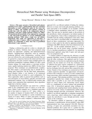
or message passing; and the C-space has no natural decomposition, leading to arbitrary partitioning schemes subjectto heuristics. In contrast, task-space approaches can usually use a workspace decomposition method as a naturalpartitioning scheme for concurrent exploration. Based onthis insight, we propose in this paper to decompose theworkspace into disjoint convex shapes. Multiple task-spaceRRT planners can thus grow the search tree in parallelwith no synchronization, each planner extending the treewithin its own convex free-space. Furthermore, this approachmakes it possible to explore the same task-space region fordifferent configuration subspaces, which greatly increasesthe robustness of the overall planner compared to globaltask-space tree approaches, such as [5], as we show in thecomparison section (Section IV).Our goal is to obtain a planner that solves real-world pathplanning problems efficiently even in the case of robots withvery high dimensionality, such as humanoid robots or serialchain approximations to soft, deformable manipulators. Tothis end, we introduce a hierarchical path planner consistingof multiple local task-space RRT planners running in parallel,and a global planner that uses the free-space connectivityinformation for coordinating the local planners.The rest of this paper is organized as follows: we formalizethe path planning problem in Section II, and describe ourpath planning algorithm in detail in Section III. A comparison with state-of-the-art planners for several examples ispresented in Section IV. Conclusions are drawn in Section V.II. P ROBLEM F ORMULATIONIn this section, we formalize the path planning problem forserially connected manipulators in two- or three-dimensionalworkspaces. Let d denote the dimensionality of the physicalspace Rd containing the workspace, d {2, 3}. In this space,a convex polytope V is a set of pointsV {x Rd Ax 6 b}, A Rn d , b Rn ,(1)which is called bounded if it is contained in a ball of finiteradius (i.e., c Rd , r R 0 , x V : kx ck r).Convex bounded polytopes are also called convex polygonsin 2D, and convex polyhedra in 3D. This paper only usesconvex and bounded polytopes, for brevity they will besimply referred to as polytopes hereafter.For the path planning problem, the robot workspace Wis considered to be a polytope. The workspace contains aOset of obstacles {Ok }nk 1, which are themselves polytopes.Obstacles that are not polytopes (e.g., spheres) can be modeled as polytope overapproximations (e.g., a dodecahedron),and non-convex shapes can be modeled as a set of polytopesthrough convex partitioning.The union of all obstacles isS nOdenoted by O O,k 1 k and the free workspace byFW W \ O.This paper considers serially connected manipulators,whose kinematics are uniquely determined by a vectorq Rnq of joint positions (angles for rotational joints anddisplacements for prismatic joints). The subset of the spaceoccupied by the robot for a specific configuration q isindicated by B(q) Rd . Let fp : Rnq Rd be the forwardkinematics function for computing the end-effector positionp Rd , i.e., p fp (q).We denote by Rnr the task-space of the path planningproblem, and by fr : Rnq Rnr a function mapping a configuration q to a task-space point r Rnr , i.e., r fr (q).In this work, the path planning problem is constrained onlyby the kinematic model of the manipulator and the staticobstacles in the environment. We further assume that wecan always find the end-effector position p for a task-spacepoint r via a function gp : Rnr Rd , i.e., p gp (r). Asan example, the task-space consisting of the position andorientation of the end-effector fulfills the criteria introducedabove. Formally, we define the path planning problem as atuple (qb , rg ), where qb Rnq is the initial configurationof the robot, and rg Rnr represents the goal point in thetask-space. A solution to the path planning problem (qb , rg )is a continuous function q(s) : [0, 1] Rnq that fulfills thefollowing conditions:q(0) qb ,fr (q(1)) rg ,(2) s [0, 1] : B(q(s)) FW .For a solution q(s), p(s) fp (q(s)) denotes the endeffector trajectory. The total length of the solution path q(s)is denoted by lq , the total length of the end-effector trajectoryp(s) by lp , and t is the duration of the planner’s execution.Intuitively, the planner should find solutions with low valuesfor t, lq , and lp ; these values are later used to compare theproposed planner with other state-of-the-art approaches.III. PATH P LANNING A LGORITHMThe path planner proposed in this work consists of aglobal planner guiding the search by using information aboutthe workspace topology, and multiple parallel local plannersconstructing collision-free paths in the task-space. The globalplanner partitions the free workspace FW into a set ofFFdisjoint polytopes F {Fi }ni 1, such that ni 1Fi FW ,and constructs a polytope adjacency graph with the polytopesF as graph vertices. Using this information, the plannercreates and maintains two trees: a task-space tree T , in which each node t (r, Q)consists of a task-space point r Rnr , and a setof configurations Q {q Rnq fr (q) r},1 i.e., allconfigurations in Q map to r; a polytope tree N , in which each node n (F, TF )consists of a free-space polytope F F, and a subsetof the task-space tree TF T with the property thatall nodes in TF correspond to end-effector points in F( t TF , gp (t.r) F ).2The local planners are used by the global planner to findcollision-free paths between adjacent free-space polytopes.Figure 1 presents a 2D path planning problem for a 6 DoFrobot, which we use hereafter to explain the algorithm.1 Notethat in [5], the tree nodes have the form t (r, q). (dot) operator is used to identify individual members of a treenode. Here, t.r denotes the task-space point r corresponding to the node t.2 The
(a) Example path planning problem(b) End-effector path (green) andexpanded task-space RRT (blue)(c) Robot pathFig. 1: Hierachical Planner solving a 2D path planning problem for a 6 DoF robot(a) Free-space partitioning(gray: free space, red: obstacle)(b) Boundaries between adjacentpolytopes (green)(c) Adjacency graphFig. 2: Data structure for the global planner: Convex decomposition and adjacency graphA. Global PlannerThe global planner (Algorithm 1) starts by partitioning thefree workspace FW into a set of disjoint polytopes F (line 1)using the binary space partitioning algorithm, introducedinitially for computer graphics in [21], and used in [14]in the context of motion planning for a mobile robot ina 2D environment. The execution time for the partitioningalgorithm is O( L 2 ) [22], where L is a set containingall facets of all workspace obstacles. The result of thepartitioning algorithm for the example workspace is shownin Fig. 2a, where the free-space polytopes are labeled usingthe numerals 1 to 5. Using the convex decomposition F, theplanner constructs a polytope adjacency graph AF (line 2),with the elements of F as vertices (Fig. 2c). The plannerchecks all pairs of polytopes and connects the correspondinggraph vertices by an edge if the polytopes have co-planarfacets whose intersection is not empty (Fig. 2b shows theboundaries for the example workspace). After finding theinitial end-effector point pb (line 3) and the correspondingpolytope Fb (line 4), the global planner initializes the rootnodes of the trees T and N (lines 5 and 6, respectively). Inour example, Fb is polytope 5, and the goal point is insidepolytope 2. The global planner starts the search at the rootnode of the polytope tree (line 7).Algorithm 1 Global planner algorithmInput: FW , (qb , rg )Output: q(s)1: F PARTITION (FW )2: AF A DJACENCY G RAPH (F)3: pb fp (qb )4: Fb F IND P OLYTOPE (F, pb )5: troot (pb , {qb }). task-space tree root node6: nroot (Fb , {troot }). polytope tree root node7: q(s) F IND PATH (nroot ). start searchGiven a polytope tree node n, the F IND PATH function(Algorithm 2) starts parallel local planners for each adjoiningpolytope Fn of the polytope n.F , attempting to find acollision-free path moving the end-effector from n.F towardsFn (lines 2 and 3). In our example, the global plannerstarts two local planners, one for connecting polytope 5 withpolytope 2, and, in parallel, one for connecting polytope5 to polytope 3. When a polytope Fn is reached, a newnode nnew is created and added to the polytope tree N ,and F IND PATH is called for the new node (lines 4 to 7). Ifthe current polytope n.F contains the goal point rg , a localplanner is started asynchronously with a ball of radius rgoal
Algorithm 2 F IND PATH ion F IND PATH(n)for Fn AF .neighbors(n.F ) do paralleltnew C ONNECT R EGION(n.TF , n.F, Fn , ρF )nnew (Fn , {tnew })n.children n.children {nnew }F IND PATH(nnew )end forif gp (rg ) n.F then parallelG BALL(rg , rgoal ). define goal regiontg C ONNECT R EGION(n.TF , n.F, G, ρgoal )qg S AMPLE(tg .Q)q(s) BACKTRACK(qg ). create solutionreturn q(s)end ifend functionaround the goal point as the target region (lines 8 to 10). Inour example, the local planner can easily find a path frompolytope 5 to polytope 2, for which a node is created inthe polytope tree. As polytope 2 contains the goal point rg ,the global planner starts a local planner inside polytope 2 tofind the path to the goal. However, the robot cannot reachthe goal point moving directly from polytope 5 to polytope2 due to the obstacles, so the algorithm continues expandingthe polytope tree until it constructs the sequence (5, 3, 4, 2),which the end-effector can follow to the goal (Fig. 1b and1c). When the goal is reached, the solution is obtained bygenerating a continuous function q(s) from the sequence ofconfigurations connecting the start qb with goal qg (lines 11to 13). The solution is returned immediately by the globalplanner, and the planner terminates. A simplified view ofthe resulting trees N and T is shown in Fig. 3; the polytopenodes n are shown as rectangles labeled with the numeralcorresponding to the free-space polytope n.F , while the taskspace nodes t are shown as dots within the polytope nodes.Note that there are two nodes corresponding to the polytope2, one for the sequence (5, 2), the other for the sequence(5, 3, 4, 2).The global planner is equivalent to a breadth-first searchalgorithm in the adjacency graph. Due to this behavior,the number of local planners running in parallel mightgrow exponentially, which can become a critical factor inexpansive environments. This problem is mitigated by severalfactors. First, we consider workspaces for robotic manipulators with a fixed base, which tend to have simpler topologiesthan workspaces for mobile robots. Second, our workspacedecomposition implementation tries to reduce the numberof resulting polytopes, thereby simplifying the topology ofthe adjacency graph. Third, we prevent the obvious casewhen the end-effector returns to the previous polytope. Forexample, in Fig. 2, after finding the path from polytope 5to polytope 3, the global planner starts two local planners,one for connecting polytope 3 to polytope 1, the other forconnecting polytope 3 to polytope 4 (no planner is started forFig. 3: Polytope and task-space trees after finding the pathto the goal (blue: start point, magenta: goal, green: solution)connecting polytope 3 to polytope 5, as these polytopes arealready connected). Fourth, we schedule the execution of thelocal planners explicitly, giving priority to more successfullocal planners, and to planners exploring shorter paths inthe adjacency graph. We give additional details about thescheduling process below.Let J be the set of active local planners at a given momentin time, Js J the set of planners that have been scheduledat least once, and Ju J the set of planners that have notbeen scheduled. As an example, assume that Js containsthe local planner connecting the goal via the sequence (5, 2)and a local planner exploring the sequence (5, 3, 4). The setJu contains two planners, one for the sequence (5, 3, 1),the other for (5, 2, 4). For each planner in Js , we countthe total number of times the planner failed to expand thetask-space tree T towards the target region (exploitationfailures), which we denote by nf ail . We choose plannersin Js randomly with a probability proportional to 1/nf ailso that more successful planners have a higher probabilityof being selected. In our example, the local planner for thesequence (5, 3, 4) has a higher probability of being selectedbecause the other planner cannot make progress towards thegoal, which increases its nf ail value. For each planner in Ju ,we estimate the end-effector path to the goal point pg usingthe information from the adjacency graph. The schedulerselects with probability ρnewpath the planner from Ju withthe shortest estimated path length (in our example, this is(5, 3, 1)), or with probability 1 ρnewpath a planner fromJs . The selected planner is assigned to one of the availableexecution threads for a limited amount of time. If the localplanner cannot solve its task within the allocated time, itis paused, and the scheduler selects another planner. Thisapproach balances the breadth-first search in the adjacencygraph with depth-first scheduling of the local planners.
Algorithm 3 Local planner ion C ONNECT R EGION(TR , R, Rnew , ρ)repeatif S AMPLE([0,1]) ρ thenrnew S AMPLE(Rnew ). exploitationelsernew S AMPLE(R). explorationend iftnear argmint TR kt.r rnew ktnew E XTEND(tnear , rnew )if tnew .r R thenTR TR {tnew }end ifuntil tnew .r Rnew. reached target regionreturn tnewend functionB. Local PlannerThe local planner algorithm (Algorithm 3) extends theTask-Space RRT algorithm introduced in [5] with obstacleavoidance and explicit null-space exploration. Given a taskspace region R Rnr , and a set of tree nodes TR T withthe property that all nodes in TR correspond to points in R( t TR , t.r R), the local planner extends the tree (lines8 to 12) until it reaches the target region Rnew Rnr (line13). We assume that R and Rnew are adjacent regions inRnr , i.e., R Rnew 6 ; the global planner ensures thatthis property holds for all calls to C ONNECT R EGION. Theparameter ρ denotes the probability of sampling the nextpoint from the target region Rnew .Given the node tnear and the new sample rnew , theE XTEND function (Algorithm 4) selects randomly a configuration qnear from tnear .Q (line 2), and computes astep towards rnew of maximum length δr (lines 3 to 6).The function AVOID O BSTACLES (called in line 8) finds theclosest robot joint to the workspace obstacles, and uses aJacobian pseudoinverse method to create a vector qavoidthat moves the joint away from the closest obstacle. AsAVOID O BSTACLES is a potentially expensive function, weonly call it with probability ρavoid (line 7). Finally, wecompute the C-space step q using the task Jacobianpseudoinverse J† , and projecting qavoid in the task nullspace (line 12). If the C-space step is unsuccessful (verifiedby collision checking in Algorithm 5, line 6), a randomself-motion step is attempted (lines 15 to 17). Exploringthe null-space explicitly through self-motion provides morepossibilities for finding collision-free paths when comparedto approaches where a single configuration is used for eachtree node (e.g., Task-Space RRT in [5]).C. Properties of the proposed path plannerThe proposed path planner has several important characteristics. First, we define the local planner to run on asubset TR of the complete tree T . This enables runningmultiple local planners in parallel, with little synchronizationAlgorithm 4 E XTEND :18:19:20:21:22:23:24:25:26:27:28:29:function E XTEND(tnear , rnew )qnear S AMPLE(tnear .Q) r rnew tnear .rif k rk δr then r. limit task-space step size r δr k rkend ifif S AMPLE([0,1]) ρavoid then qavoid AVOID O BSTACLES(qnear )end ifJ JACOBIAN(qnear )J† JT (JJT ) 1 q J† r (I J† J) qavoidqnew QS TEP(qnear , q)if qnew then. explore null spaceqrandom S AMPLE(Rnq ) q (I J† J)(qrandom qnear )qnew QS TEP(qnear , q)if qnew 6 thenqnear .children qnear .children {qnew }tnear .Q tnear .Q {qnew }end ifreturn elseqnear .children qnear .children {qnew }tnew (fr (qnew ), {qnew })tnear .children tnear .children {tnew }return tnewend ifend functionAlgorithm 5 QS TEP algorithm1:2:3:4:5:6:7:8:9:10:11:function QS TEP(q, q)if k qk δq then q q δq k qkend ifqnew q qif B(qnew ) FW thenreturn qnewelsereturn end ifend function. limit c-space step size. collision checkingneeded, which greatly improves the performance of the overall planner. Second, partitioning the free-space into convexpolytopes implies that the line connecting any two pointswithin a polytope does not intersect any obstacles. Thus,because the end-effector cannot collide with the workspaceobstacles, the local planner can use higher probabilities ρof sampling in the target region compared to typical valuesused by global RRT planners to sample the goal point. Thismeans that our path planer focuses more on exploitationthan exploration, and can potentially find the solution ina shorter time. Third, the global planner creates different
polytope nodes n for a polytope found through differentsequences (Algorithm 2, line 4), which means that multiplelocal planners can grow the task-space tree T within thesame polytope without interfering with each other. Thelocal planners are thus exploring different subspaces of theconfiguration space. This approach ensures that our planner’srobustness is significantly better compared to global taskspace RRT, and comparable or better than that of C-spaceplanners, as shown in the next section. Fourth, polytopesequences containing cycles are permitted, which enables theexploration of different configuration subspaces in previouslyvisited regions of the workspace. As an example, consider thepath planning problem shown in Fig. 4a, where the plannerneeds to retract the end-effector on a path around the bottomright obstacle, then pass again through the central region toreach the goal in the top-left corner. This characteristic isa significant advantage both over hierarchical path plannersthat use cycle-free paths in the adjacency graph (found viashortest path algorithms), such as the approach in [17], andglobal task-space planners like [5], where the tree expansioncan prevent the planner from finding a solution (see Fig. 4d).An important topic when introducing new sampling-basedpath planning algorithms is the notion of probabilistic completeness. A path planning algorithm is probabilisticallycomplete if, assuming a feasible path exists, the probabilityof finding the solution approaches one as the computationtime goes to infinity. While being mathematically useful, ithas been argued [12] that the definition has little practicalvalue for real-world path planning problems, where thecomputation time going to infinity is not an option. A moreuseful notion would be the probability of finding a solutiongiven a finite amount of time, although this might be difficultto estimate. Similar to the approach in [12], our path planningalgorithm values computational efficiency over probabilisticcompleteness.IV. A PPLICATION EXAMPLES AND COMPARISONSThe performance and robustness of the proposed hierarchical planner is tested in several different scenarios, andcompared to different state-of-the-art path planning algorithms. The following examples were selected to illustratethe advantages and drawbacks of the proposed planner:3 A 2D workspace containing 4 square obstacles, with a100 DoF manipulator that approximates a flexible robot(Fig. 4). A 3D workspace containing a wall with 4 square holes,and an 8 DoF manipulator. The robot starts with the endeffector inside the top-left hole, and needs to enter oneof the bottom holes to reach the goal position (Fig. 5). A 3D workspace where a humanoid robot needs to reachwith the right hand the content of a box placed on topof a table. The kinematics is modeled after TORO [23],a 27 DoF humanoid robot developed at DLR. For thisexample, the torso is not connected to the waist, andcan rotate freely in three dimensions. Together with3 theattached video shows more application examples.the 6 DoF arm, it creates a 9 DoF robotic manipulator(Fig. 6).The planner proposed here (Hierachical Planner) is compared with four other planners: RRT-Connect with one tree(RRT-Connect) [4], RRT-Connect with two trees (BiRRTConnect) [4], an adaptive dynamic-domain RRT with twotrees (ADD-RRT) [24], and a task-space RRT with oneglobal tree (TS-RRT) [5], which we modified to use thesame task-space RRT structure as our local planner, andthe E XTEND function presented in Algorithm 4. For theseplanners, the nearest neighbor search was implemented usingkd-trees [25], with the parameter k 30. In order to ensure afair comparison, as our hierarchical planner was designed fora multi-threaded execution, we implemented multi-threadedvariants of the mentioned algorithms, and configured themto use the same number of execution threads as our planner.For all planners, the solution returned by the planner is firstsimplified using an iterative approach that finds shortcuts inthe configuration sequence, and then smoothed to create aquadratic Bézier curve.All planners are implemented in Java, and the exampleswere executed on a standard Windows PC with 3.5 GHzIntel Xeon processor and 8 GB of RAM. Collision detectionand distance queries were performed using a proprietaryimplementation. The results are averaged over 100 trials; ifa planner does not solve the problem within 30 seconds, thetrial is considered a failure and the planner is stopped. Thetables in Fig. 4 to 6 show the mean value and the standard deviation of the following values (only considering successfultrials): execution time t, number of collision checks, C-spacepath length lq (using Euclidean norm), and end-effector pathlength lp . The last column shows the percentage of successfultrials. Accompanying images show one trial result for thefour different planners; BiRRT-Connect was omitted as theresults are very similar to ADD-RRT.For all planners, we used the following common parameters: number of execution threads nthreads 6, goal radiusrgoal 0.005 m, maximum C-space step δq 0.1, andmaximum task-space step δp 0.025 m. For our hierarchical planner, we used the following parameters: ρgoal 0.5(probability of sampling the goal region), ρF 0.9 (probability of sampling in the neighboring polytope), ρavoid 0.5(probability of adding collision avoidance in the E XTENDfunction), ρnewpath 0.3 (probability of selecting a localplanner which explores a new path). These values wereempirically chosen to maximize the performance using Fig. 6as an archetypal example. For the other single tree planners(RRT-Connect and TS-RRT), the probability of samplingthe goal was set to ρ 0.25. Note that the free-spacepartitioning in the proposed planner makes it possible to usehigher probabilities for sampling the local goal (ρgoal andρF compared to ρ), which means that the planner focusesmore on exploitation than exploration.The first example from Fig. 4 shows the advantage of thetask-space over the C-space RRT in the case of a high-DoFmanipulator (100 DoF here). The bidirectional planners onlymanage to solve the path planning problem in 49% of the
(a) Hierarchical PlannerPlannerHierachical PlannerADD-RRTBiRRT-ConnectRRT-ConnectTS-RRT(b) ADD-RRTTime (s)4.70 1.2518.31 7.3718.69 8.04N/AN/ACollision Checks34281 1192662625 1830562874 21273N/AN/A(c) RRT-Connectlq3.498 0.22114.197 1.55114.710 1.943N/AN/A(d) TS-RRTlp (m)1.830 0.0642.197 0.2562.296 0.297N/AN/ASuccess (%)100493700Fig. 4: 2D workspace example with 100 DoF robot(a) Hierarchical PlannerPlannerHierachical PlannerADD-RRTBiRRT-ConnectRRT-ConnectTS-RRT(b) ADD-RRTTime (s)1.39 0.402.42 0.792.64 0.94N/A6.33 4.84Collision Checks7675 504918809 1011721637 14349N/A147262 121840(c) RRT-Connectlq5.147 0.18113.986 3.63113.937 3.981N/A4.706 0.125(d) TS-RRTlp (m)1.
geometry [9], the medial axis of the free workspace [10], or spherical free-space regions computed on a generalized Voronoi graph [11]. An alternative approach is to partition the free workspace into cells, and use their connectivity infor-mation. Tunnels of free workspace are constructed in [12] by a sphere expansion algorithm. An approximate .