Transcription
Lab 3 Sample Notebook%pylab inline#%pylab notebook#%matplotlib qtimport sk dsp comm.sigsys as ssimport scipy.signal as signalimport ipywidgets as widgetsfrom ipywidgets import interact, interactive, fixed, interact manualfrom IPython.display import Audio, displayfrom IPython.display import Image, SVGPopulating the interactive namespace from numpy and matplotlibpylab.rcParams['savefig.dpi'] 100 # default 72#pylab.rcParams['figure.figsize'] (6.0, 4.0) # default (6,4)#%config InlineBackend.figure formats ['png'] # default for inline viewing%config InlineBackend.figure formats ['svg'] # SVG inline viewing#%config InlineBackend.figure formats ['pdf'] # render pdf figs for LaTeX# div style "page-break-after: always;" /div #page breaks after in TyporaSupport Functionsdef line spectra dBm(fn,Xn,floor dBm -60,R0 50,lwidth 2):"""Plot the one-sided line spectra from Fourier coefficients in dBm.Inputs-----fn harmonic frequencies correspinding to Xn'sXn pulse train FS coefficientsfloor dBm spectrum floor in dBmR0 impedance (default 50 ohms)Returns------Sx dBm One-sided bandpass lines as dBm levelsMark Wickert February 2019"""Lab 3 Notebook SamplePage 1 of 12
Xn dBm abs(Xn*sqrt(1000/(2*R0)))Xn dBm[0] abs(Xn[0])*sqrt(1000/(R0))ss.line spectra(fn,Xn dBm,mode 'magdB',sides 1,lwidth lwidth,floor dB floor dBm)ylabel(r'Power (dBm)')xlabel(r'Frequency (Hz)')title(r'Line Spectra PSD')Sx dBm 20*log10(2*Xn dBm)Sx dBm[0] - 6.02return Sx dBmDouble Balanced Mixer ModelingConsider both LTSpice and a behavioral level model in Python.LTSpice DBM Circuit SimulationImport time domain and spectrum results from a simplified DBM circuit simulation.# Skip the first 32 rows, then skip the last row that contains 'END't spice, RF out loadtxt('DBM mod time.csv',delimiter ',',skiprows 1,usecols (0,1),unpack True)plot(t spice[:3200]*1e6,RF out[:3200]*1e3)title(r'LTSpice Simplified DBM Time Domain Output x {RF}(t) ')ylabel(r'Amplitude (mV)')xlabel(r'Time ( \mu s)')grid();Lab 3 Notebook SamplePage 2 of 12
# Skip the first 32 rows, then skip the last row that contains 'END'f spice, RF out psd loadtxt('DBM mod spec.csv',delimiter ',',skiprows 1,usecols (0,1),unpack True)plot(f spice/1e6,RF out psd)title(r'LTSpice DBM Spectrum of x {RF}(t) at 10 MHz with 100 kHz Mix')ylabel(r'Power Spectrum (dBm?)')xlabel(r'Frequency (MHz)');ylim([-110,-30])xlim([5,80])grid();Lab 3 Notebook SamplePage 3 of 12
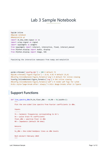
Python Behavioral Level ModelingThe behavioral level model is motivated by the understanding that the mixer high level signal, typically theLO port, drives the diode ring into switching mode. The LO signal then appears approximately as a squaredwave signal multiplying the low level input signal at the IF port or RF port. The first step in development ofthis model is to understand a diode clipper built using Schottky diodes.Soft Limiter and a Diode Clipping ModelUse thefunction to approximate the soft clipping action of the Schottky diode ring found in theDBM.First consider the input/output characteristic:x arange(-5,5,.01)for k in range(4):alpha [4,6,10,100]y r'Soft Limiter Created with y \arctan(x\alpha) ')ylabel(r'Output Voltage')xlabel(r'Input Voltage')legend((r' \alpha 4 ',r' \alpha 6 ',r' \alpha 10 ',r' \alpha 100 '))grid();Lab 3 Notebook SamplePage 4 of 12
Simulate the simple diode clipper in LTSpice when driven by a single sinusoid. LTSpice simulation results areimported and then a reasonable value is chosen for a 7 dBm LO drive sinuoid.# Skip the first 32 rows, then skip the last row that contains 'END't clip, clip out loadtxt('DiodeClipper.csv',delimiter ',',skiprows 1,usecols (0,1),unpack True)# Behavioral level model using arctan as an amplitude limitert behav arange(0,1e-3,1e-5)x behav 1.416*sin(2*pi*2000*t behav)y behav arctan(x behav*4.0)*2/piy behavs y behav*max(clip out)/max(y behav)plot(t behav*1e3,y behavs)plot(t clip[:-1]*1e3,clip out[:-1])title(r'Fitting the \arctan() Model to the DBM Circuit')ylabel(r'Amplitude (V)')xlabel(r'Time ( \mu s)')legend((r' \arctan Model',r'LTSpice Schottky Clipper'))#ylim ([-.4,.4])grid();Lab 3 Notebook SamplePage 5 of 12
From the above we see thatis a good fit for the 7 dBm LO input. Define the DBM model withfunction DBM model() having parameters alpha to control the soft limiter threshold and conv loss tomodel the mixer conversion loss from the low level input relative to the desired sum and differencefrequency outputs. Understand that the loss reflects the fact that the mixer converts the input signal IF/RFto additional output frequencies (harmonic and intermod terms).def DBM model(x LO,x IF RF,conv loss dB 5.0, alpha 4.0, ):"""Mark Wickert February 2019"""x LO clip 10**(-conv loss dB/20)*arctan(x LO*alpha)*2/pix IF RF clip 10**(-conv loss dB/20)*arctan(x IF RF*alpha)*2/pix out x LO clip*x IF RF clipreturn x out, x LO clip, x IF RF clipA Quick SimulationWe will later calculate approximate Fourier series coefficients in order to plot the power spectrum. WithMHz andkHz, we know that x RF will be periodic with period of 1/100e3 10 s.Thus in the following simulation we choose a sampling rate of 1 GHz for a high fidelity waveform and asimulation period of 10 s.t arange(0,10e-6,1e-9)x LO 1.416*cos(2*pi*10e6*t)x IF 0.0632*sin(2*pi*100e3*t)x RF, x LO clip, x IF clip DBM model(x LO, x IF,conv loss dB 6.5)Lab 3 Notebook SamplePage 6 of 12
plot(t*1e6,x RF*1e3)#plot(t*1e6,x LO clip*1e3)#xlim([0,1])title(r'Behavioral DBM Model Time Domain Output x {RF}(t) ')ylabel(r'Amplitude (mV)')xlabel(r'Time ( \mu s)')grid();Xk, fk ss.fs coeff(x RF,550,100e3)Xn dBm line spectra dBm(fk/1e6,Xk,-80,lwidth 1)title(r'DBM Behavioral Model x {RF}(t) Line Spectrum')xlabel(r'Frequency (MHz)');ylim([-80,-10])xlim([5,55]);Lab 3 Notebook SamplePage 7 of 12
for k, Xn dBm k in enumerate(Xn dBm):if Xn dBm k -50: # Threshold -30 dBmprint('Peak at %6.4f MHz of height %6.4f dBm'% (fk[k]/1e6,Xn dBm[k]))PeakPeakPeakPeakPeakPeakatatatatatat9.9000 MHz of height -24.4505 dBm10.1000 MHz of height -24.4505 dBm29.9000 MHz of height -37.0442 dBm30.1000 MHz of height -37.0442 dBm49.9000 MHz of height -44.5326 dBm50.1000 MHz of height -44.5326 dBmMeasurement Example atMHz andkHz# Skip the first 32 rows, then skip the last row that contains 'END't scope, scope ch1, scope ch2 loadtxt('scope dbm mod.csv',delimiter ',',skiprows 2,usecols (0,1,2),unpack True)Lab 3 Notebook SamplePage 8 of 12
def my find(condition):"""Find the indices where condition is true in an ndarrayMark Wickert February 2019"""idx np.nonzero(np.ravel(condition))[0]return idx(my find(t scope 0), my find(t scope 10e-6))(array([902]), array([1902, 1903, 1904, 1905, 1906]))plot(t scope[902:1902]*1e6,scope ch1[902:1902]*1e3)title(r'Scope Measured Output x {RF}(t) ')ylabel(r'Amplitude (mV)')xlabel(r'Time ( \mu s)')grid();Lab 3 Notebook SamplePage 9 of 12
# Skip the first 32 rows, then skip the last row that contains 'END'f SA, Sx DBM mod 10M 100k loadtxt('DBM MOD 10M 100K.csv',delimiter ',',skiprows 32,usecols (0,1),comments 'END',unpack True)plot(f SA/1e6,Sx DBM mod 10M 100k)xlabel(r'Frequency (MHz)')ylabel(r'Power Spectrum (dBm)')title(r'FieldFox 10 MHz LO, 7dBm, 100 kHz IF, -20 dBm')ylim([-70,-20])xlim([5,35])grid()peak idx signal.find peaks(Sx DBM mod 10M 100k,height (-75,)) # peak threshold -30 dBmfor k, k idx in enumerate(peak idx[0]):print('Peak at %6.4f MHz of height %6.4f dBm'%(f SA[k idx]/1e6,Sx DBM mod 10M 100k[k idx]))Lab 3 Notebook SamplePage 10 of 12
atat9.8750 MHz of height -24.5360 dBm10.1250 MHz of height -24.5541 dBm20.0000 MHz of height -59.8962 dBm29.8750 MHz of height -35.2565 dBm30.1250 MHz of height -35.2895 dBm39.8750 MHz of height -66.5790 dBm40.1250 MHz of height -66.2963 dBm49.8750 MHz of height -41.4309 dBm50.1250 MHz of height -41.4799 dBmMore accurate frequency location can be obtained via spectral zooming and/or a smaller resolutionbandwidth.Lab Tasks Work AreaCharacterizing the Power Splitter Combiner# Skip the first 13 rows assuming tab spacing between entriesf s2p, S11magdB,S11deg,S21magdB,S21deg loadtxt('ADP 2 1 SUM2P1.s2p',delimiter '\t',skiprows 13,usecols (0,1,2,3,4),unpack True)plot(f s2p/1e6,S21magdB)xlabel(r'Frequency (MHz)')ylabel(r' S {21} 2 (dB)')title(r'Power Splitter Sum Port to Port 1 ( S {21} dB)')ylim([-6,0])grid();# Skip the first 13 rows assuming tab spacing between entriesf s2p, S11magdB,S11deg,S21magdB,S21deg loadtxt('ADP 2 1 ISO P1 P2.s2p',delimiter '\t',skiprows 13,usecols (0,1,2,3,4),unpack True)plot(f s2p/1e6,S21magdB)xlabel(r'Frequency (MHz)')ylabel(r' S {21} 2 (dB)')title(r'Power Splitter Port 1 to Port Isolation ( S {21} dB)')ylim([-40,0])grid();Mixer BasicsDouble Sideband Modulation and DemodulationPart dLab 3 Notebook SamplePage 11 of 12
fs 100e6 # sampling ratefc 1e6 # cutoff frequencyb, a signal.cheby1(5, 1, 2*fc/fs) # digital filter designimport sk dsp comm.iir design helper as iir hiir h.freqz resp list([b],[a],'dB',fs/1e3)ylim([-80,0])grid();fc 5e6fm 100e3t arange(0,2/(100e3),1/100e6) # Two cycles of 100 kHz with fs 100 MHz# Create the modulated DSBx LO 1.416*cos(2*pi*fc*t)x IF 0.0632*sin(2*pi*fm*t)x RF, x LO clip, x IF clip DBM model(x LO, x IF,conv loss dB 5.0)# Create the coherently demodulated DSB# Write code here.x demod .# Filter with 1 MHz LPFy demod signal.lfilter(.)plot(t/1e3,y demod*1e3) # t in ms and V in mVAM Modulation and DemodulationPart cBring scope and LTSpice results together.Lab 3 Notebook SamplePage 12 of 12
Lab 3 Sample Notebook Suppor t Functions %pylab inline #%pylab notebook #%matplotlib qt import sk_dsp_comm.sigsys as ss import scipy.signal as signal import ipywidgets as widgets from ipywidgets import interact, interactive, fixed, interact_manual from IPython.display import Audio, display from IPython.display import Image, SVG