Transcription
WP/04/6A Puzzle of Microstructure Market MakerModelsRafael Romeu
2004 International Monetary FundWP/04/6IMF Working PaperInternational Capital Markets DepartmentA Puzzle of Microstructure Market Maker ModelsPrepared by Rafael Romeu1Authorized for distribution by Donald J. MathiesonJanuary 2004AbstractThis Working Paper should not be reported as representing the views of the IMF.The views expressed in this Working Paper are those of the author(s) and do not necessarily representthose of the IMF or IMF policy. Working Papers describe research in progress by the author(s) and arepublished to elicit comments and to further debate.This study addresses the empirical viability of microstructure models of dealer price setting.New evidence is presented rejecting these models’ specifications of how informationasymmetry and inventory accumulation affect dealer pricing. This rejection is consistentwith those of other dealer-level empirical studies. This study suggests a new modelingoption may be to reconsider optimal price setting while relaxing assumptions that specifyincoming orders as the only component through which dealer inventories evolve. Thisapproach is consistent with inventory evolution data and with general equilibrium models’assumptions about currency markets.JEL Classification Numbers: C52; G15; F31Keywords: Foreign Exchange, Microstructure, Inventory, Information, Market MakersAuthor’s E-Mail Address: rromeu@imf.org1I am grateful to Roger Betancourt, Michael Binder, Robert Flood, Carmen Reinhart, and John Shea for guidance;I am grateful to Richard K. Lyons for data and guidance. Thanks to two anonymous referees, Richard Adams,Juan Blyde, David Bowman, Alain Chaboud, Andrew DePhillips, Larry Evans, Martin Evans, Jon Faust,Stefan Hubrich, Andrei Kirilenko, Don Mathieson, José Pineda, Matt Pritsker, John Rogers, Francisco Vázquez,Jonathan Wright, Citibank FX, the Board of Governors of the Federal Reserve, the University of MarylandEconomics Department, and the R. H. Smith School of Business for many valuable comments and suggestions.I am also grateful to Jushan Bai for code. The views expressed are not necessarily shared by the aforementioned;all errors and omissions are my own.
-2-ContentsPageI.Introduction. 3II.Reconsidering the Lyons (1995) Result. 6III.A Puzzle of Microstructure Market Maker Models. 9IV.Conclusion . 11References. 21Figures1.2.3.4.5.Partitions in the Exchange Rate Literature .13Rolling Estimates of Break Tests and DL Pricing Equation. 14Price, Daily Cumulative Components of Inventory, and Breaks. 15Kernel Density Plots for QQit and Qjt . 16Impulse Responses for QQit and Qjt . 16Tables1.2.3.4.5.6.7.8.Reproduction of Lyons (1995) Original Estimates. 17Sup-F Tests for Location and Number of Structural Breaks . 17Break Test for Fed Intervention. 18Estimates DL Pricing Model in Subsamples with no Breaks . 18First Five Entries of Lyons (1995) Dataset. 19Descriptive Statistics for QQit and Qjt . 19VAR Lag Order Selection Criteria .20Vector Autoregression Estimates.20
-3-I. IntroductionExchange rate models that reflect information gathering and risk sharing in theircurrency-trading processes have recently shown empirical success. In these models(often referred to as micro exchange rate models), the exchange rate depends not just ontracked statistics of economic aggregates, such as inflation or investment, but also onother variables that reflect the market’s view of economic conditions. One can partitionmicro exchange rate models into general equilibrium models and dealer-level models.General equilibrium (GE) micro exchange rate models study how a market-wideconsensus of asset values is achieved. GE models focus on how the entire market buildssuch a consensus and settles on an exchange rate. These models can explain more than50 percent of exchange rate movements.2 Dealer-level (DL) micro exchange rate modelsabstract from the market as a whole and instead focus on price setting and riskmanagement by individual currency market participants, or dealers. This study exploresa rift between GE models and DL models. First, it shows new empirical rejections ofsome DL model predictions. Next, it shows that a basic DL assumption is inconsistentwith GE models and with the data. This may be the reason that some DL modelpredictions are routinely rejected both in this and previous studies.Before explaining the difficulties with DL models put forth here, it is useful tomap exactly where they lie in the literature of exchange rates. Figure 1 (page 13)partitions the research on exchange rates into six broad categories. Traditional models ofexchange rates, which face well-known empirical difficulties, are represented by Box (1).In these models, a handful of parity conditions are assumed to link macroeconomicactivity across countries. One such condition is purchasing power parity (PPP). PPPrelates the difference in inflation rates across countries to their exchange ratedepreciation. Although empirical predictions of macroeconomic models are generallyinconsistent with exchange rate data, parity conditions are consistent. Specifically, Floodand Taylor (1996) show that long-run data support PPP and other parity conditions, asdenoted in Box (2). The upshot of their study is given in equation (1). Exchange ratedepreciation between two periods of time (t denotes time, e denotes exchange ratedepreciation) depends on publicly observable fundamental macroeconomic variables(denoted by F) and an “unexplained” component (denoted by U). et Ft U t(1)Instead of assuming that parity conditions govern exchange rate evolution, microexchange rate models consider factors that drive currency market participants’ pricesetting. Empirical GE micro exchange rate models, such as Evans and Lyons (2002), arerepresented in Box (4). In these models, market participants receive economicinformation through order flow that they cannot learn from public macroeconomicstatistics. Order flow results from partitioning total traded volume into either buyer2Evans and Lyons (2002a and b).
-4initiated transactions or seller-initiated transactions and taking their difference. Orderflow plays an important role in estimating the exchange rate because it captures changesin expectations and risk preferences that are absent from publicly tracked economicaggregates. The resulting exchange rate depreciation equation (2) is almost identical toequation (1). The interest rate differential change (denoted (rt rt* ) ) represents thefundamental variable, and the “unexplained” variable of Flood and Taylor (1996) is theorder flow variable (denoted xt ) in Evans and Lyons (2002). et ( rt rt* ) xt(2)The theory that yields the empirical specification in (2) is based on GE models ofsimultaneous trading in currency markets (see, for example, Lyons (1997) — Box (3) inFigure 1). In these models, first exchange rates are simultaneously set by currencydealers. These dealers must all set prices (simultaneously) at which they are willing tobuy or sell any amount of currency. Next, market participants observe everyone else’sexchange rates and submit their orders to the others in the market. These conditionsguarantee that all dealers set the same exchange rate, because any differences would leadto large arbitrage opportunities and unravel the equilibrium. In equilibrium, all dealersset the same exchange rate and there are no opportunities for arbitrage. For all dealers toknow which exchange rate to set, it must be based on publicly available information.Hence, in these models, dealers’ exchange rates are common and based on publiclyknown order flow and macroeconomic variables.Actual market participants, however, are constantly changing prices in over-thecounter currency markets. That is, since currency trading occurs over the counter, at anypoint an individual dealer’s exchange rate may diverge from others’ in the market. 3 Tostudy price setting in this market, DL models consider individual dealers’ exchange ratesetting — Box (5) in Figure 1. Dealers in these models set prices as they receiveincoming orders from other market participants. The initiators of the incoming ordersmay know more about future asset values than the dealers receiving the orders. In thissituation, the incoming orders reflect information about future asset values andconsequently drive currency prices. This is the asymmetric information effect. Also, inthese models dealers have a finite inventory of the asset on which to draw for liquidityprovision. As incoming orders drive the dealer’s asset inventory away from her optimallevel, she changes prices to induce compensating orders. This is the inventory effect.The classic DL pricing conjecture is given by Madhavan and Smidt (1991) — in Box (5)in Figure 1.3Then one may ask why the assumptions of GE models guarantee that all dealers set the same price. Thereturn in economic insight to modeling competitive dealers is likely to be small relative to the cost ofovercoming the intractability of competitive markets, particularly in terms of the necessary assumptions.See O’Hara (1995) on precisely this intractability (Chapter 2, Inventory Models).
-5Empirical tests of DL models generally support asymmetric information effects,4they do not, however, find inventory effects.5 One study, Lyons (1995), finds directevidence of asymmetric information and inventory management predicted by DLinventory theory — Box (6) in Figure 1.This study reconsiders the use of traditional dealer-level pricing specifications,and, specifically, this study reexamines the Lyons (1995) result. Evidence of parameterinstability and model misspecification in Lyons (1995) is presented. When estimatedover the full dataset, that study’s DL pricing equation contains breaks. In subsampleswhere no breaks are present, the results do not fully support DL model predictions.Specifically, asymmetric information and inventory effects are not presentsimultaneously in subsamples; and hence, although they do not reject the presence ofasymmetric information or inventory effects in the data, the models’ specifications ofthese effects are rejected. This is the subject of Section II, and is indicated by the brokenlink between Box (5) and Box (6).Section III discusses an underlying assumption in DL models’ pricingspecification that may be behind their persistent empirical difficulties. Basically, theassumption that inventory accumulation is driven only by incoming order flow isquestionable. This assumption is shown to be in contradiction to both the inventory dataand GE micro exchange rate theory. This is indicated by the broken link between Box(3) and Box (5). Relaxing this assumption is a promising avenue for further DLmodeling. Section IV concludes.4For example Hasbrouck (1988, 1991a, 1991b), Madhavan and Smidt (1991, 1993) in equity markets,Lyons (1995), Yao (1998), Bjonnes and Rime (2000) for foreign exchange markets, among others.5Madhavan and Smidt (1991) do not find inventory effects. Madhavan and Smidt (1993) allow a changingoptimal inventory level, and find evidence of inventory management with a half-life of over seven days,suggesting quite different effects from theoretical predictions. Furthermore, they reject the hypothesis ofintraday inventory management, whereas Madhavan, Richardson and Roomans (1997) argue that if there isinventory management, it occurs towards the end of the day. Hasbrouck and Sofianos (1993) find veryslow inventory adjustment as well, though they confirm that specialists are in fact able to adjust inventoryquickly during large exogenous shocks if they choose to. Hence inventory levels are voluntary, not due tovolume constraints, and must reflect long-term positions. Manaster and Mann (1996) find strong evidencethat specialists do not control inventory as models would predict, but rather the exact opposite occurs.Furthermore, Madhavan and Sofianos (1997) also find that dealers do not change quotes to induce trades astheoretically predicted, but rather participate selectively in markets to unwind undesired positions. Thegeneral empirical failure of inventory model predictions described above for equity markets is borne out inforeign exchange market studies by Yao (1998), and Bjonnes and Rime (2000). Neither study can find theinventory management results predicted by the Madhavan and Smidt (1991) model.
-6-II. Reconsidering the Lyons (1995) ResultThis section reconsiders the Lyons (1995) DL exchange rate model (for details,see that study). Equation (3) gives the Lyons (1995) DL specification for how thedealer’s price changes at each an incoming trade (denoted by subscript t). Intuitively, thechange in the exchange rate is a function of the incoming order size, direction of trade(i.e. purchase or sale), and current and past inventory levels. Pt β 0 β1Q jt β 2 I t β 3 I t 1 β 4 Dt β 5 Dt 1 ma (1) ,(3)with predicted signs: {β1 , β 3 , β 4 0}, {β 2 , β 5 0} .Pt:Qjt:It:Dt:The price of the dealer at which an incoming sale or purchase occurred.The incoming quantity demanded by the opposite party, i.e. order flow.This is the dealer’s inventory at the time of (but not including) the incomingquantity Qjt.The indicator that picks up the direction of trade, positive for purchases, negativefor sales.Equation (3) predicts increasing prices with purchase orders and larger lagged inventory,and decreasing prices with sale orders, and larger current inventory.6 The Lyons (1995)estimates of this equation are presented in Table 1 (page 17).7 The estimates areconsistent with model predictions and significant at better than one percent. Therobustness of these estimates is the subject of this section.Figure 2 (page 14) shows evidence of parameter instability in equation (3). Ineach graph, the abscissa indexes the incoming trades. The top two panels graph theprobability that the trade is a breakpoint, with P-values indicated in the ordinate (both theF-test and the Likelihood Ratio test are reported). As the graphs show, the nullhypothesis of no break is rejected towards the middle of the sample, as well as towardsthe end (the left graph uses the Chow breakpoint tests, the right uses Wald tests). This isindicated by the declining P-values throughout the middle of the sample and again at theend. The bottom panels show how the coefficients on equation (3) change as theregression is estimated on a rolling window of 150 transactions (beginning with thetransaction indicated on the abscissa). The bottom left panel graphs the coefficient on6The moving average coefficient on the error term in equation (3) is predicted negative.The data are a one week (843 observation) data set of a NY currency dealer the dollar/DM market fromAugust 3–7, 1992. See Lyons (1995) for an extensive exposition of this data set. The Lyons (1995) modelincludes a public information signal, and specification of equation (3) with an extra regressor – brokeredtrading, Bt. That study estimates (3) both with and without the public signal because of poor measurementof the public signal in relation to the measurement of the other variables. Essentially, the brokered tradingvariable has measurement error and is zero in 84 percent of the dealer’s transactions. This section focuseson estimates without brokered trading, however, a single break is found with it included in the Sup-F test.7
-7incoming order flow ( β1 ) and its t-statistic. The bottom right panel does the same for thecontemporaneous inventory coefficient ( β 2 ). While one would expect some variation inthe significance of the estimates due to a smaller sample, the variation should not besystematic and should reduce the estimates’ significance uniformly. One can observethat order flow is significant in the beginning of the sample, whereas inventory issignificant towards the end of the sample. Hence, the DL model predictions ofasymmetric information (significant order flow coefficient β1 ) and inventory effects(significant inventory coefficient β 2 ) appear to not hold in subsamples. To get a feel forwhat is occurring at these points, Figure 3 (page 15) shows the price set by the dealer.Solid vertical lines show the end of days of the week, and dashed vertical lines show twobreaks considered in this section. The declining P-values in Figure 2 come at the end ofthe third day and close to the end of the sample.To investigate the possibility of parameter instability in equation 1, Table 2 (page17) reports test the results for the presence or location of (possibly multiple) structuralbreaks.8 A break is found at transaction 449. The right column of Table 2 reports thestarting and ending observations of each of the five trading days from which the data wasrecorded. As Figure 3 shows, the break occurs near the end of Wednesday (overnightobservations are removed). This break coincides with the end of a trading day, however,with three other day changes, there is no evidence to suggest that these alone inducestructural breaks. Figure 2 suggests that there is another break towards the end of thesample, however, Sup-F tests cannot detect breaks within five percent of sampleendpoints. On the last day of the sample, a 300 million Fed intervention occurred afterthe close of the European markets.9 This event may cause further parameter instability inthe DL model estimates.10 Hence, Table 3 (page 18) reports conventional break testsconducted on the trade at which the intervention begins. The breaks and price are jointlyshown in Figure 3 (page15). Given these joint results, one may conclude that the DLmodel is subject to two breaks when estimated on the Lyons (1995) data.8Sup{F} tests based on Andrews (1993)/Bai Perron (1998).9The Federal Reserve confirms a 300 million intervention on that day, but does not reveal its interventiontiming or strategy. The financial press widely report (ex-post) the approximate intervention start. Themost precise timing is documented by the Wall Street Journal, August 10, 1992: “The Federal ReserveBank of New York moved to support the U.S. currency. as the dollar traded at 1.4720.” That pricecorresponds to 12:32 pm in the Lyons (1995) data set, and that time is consistent with other financial newsreports.10Models which show how interventions affect trading include Bhattacharya and Weller (1997),Dominguez (2003), Evans and Lyons (2001), Vitale (1999), and others. For example, Evans and Lyons(2001) model and find evidence of portfolio balance effects from interventions. A late-day and end-ofweek intervention, one that occurs after other major markets (London and Tokyo) have closed for theweekend, would presumably bring to bear these effects. That is, the dealer would have very little time andfewer market participants (since the entire market would be affected) with which to share the intervention’sportfolio imbalance over-the-weekend, and hence, charge a higher premium for liquidity provision than atother times.
-8Table 4 (page 18) reports estimations of the DL model on the subsamples thatresult from segregating the data at the breaks. Estimates from the subsample prior to thefirst break (observations 2 to 448) are in the top panel; this subsample of data representsover 53% of the available observations. The estimates reveal that the coefficients forinventory are insignificant at conventional levels, whereas signed order flow (i.e. theasymmetric information effect) and the order flow indicators are significant andestimated at magnitudes similar to the baseline estimates.The estimates from the sub-sample 449 to 794 are reported in the middle panel.The order flow coefficient is now insignificant, and the inventory components aresignificant at all conventional levels. These estimates suggest that asymmetricinformation is not present in dealer pricing on the last two days of the sample, which isjust prior to the Fed intervention.The third subsample, consisting of approximately 5 percent of the total availableobservations, likely reflects the effects of the Fed intervention. The only significanteffect (at the 10 percent level) is the asymmetric information effect, and it seems to be anorder of magnitude larger than the other subsample estimates. In general, the model fitsthis section of the sample poorly.The bottom panel shows estimates that result from joining the third subsample tothe second, essentially ignoring the Fed intervention break. The Sup-F test cannot findthis break (because of its proximity to the sample endpoint) but the Chow test does rejectthe null of no break at this point. Estimating these two subsamples jointly shows orderflow and the order flow indicator coefficients significant at the one percent level but notat ten percent. The inventory effects are significant and the signs of the coefficients areas predicted (which was not the case for the Fed intervention subsample alone).However, the proportion of variation explained by the regression falls from 32 (withoutthe intervention subsample) to 17 percent (with the intervention subsample). Hence,while the estimation that averages across the two subsamples (i.e. ignoring the Fedintervention) recuperates to some extent DL model predictions, adding observationsreduces its explanatory power. Furthermore, identifying the first break at the first or lastobservation at which the Chow test p-value falls below 5 percent in Figure 2(observations 392 and 541) does not change the result that the first regime does not haveinventory effects, and the second has no asymmetric information effects.
-9-III. A Puzzle of Microstructure Market Maker ModelsDL models study the transaction prices that currency dealer set as orders arrivethroughout the trading day. They draw from equity market studies, which consider a theprice setting behavior of an equity market specialist. Consistent with specialists’inventory management theory,11 DL models assume that dealers set prices to control aninventory that evolves according to equation (4)12:I it 1 I it Q jt ,(4)with I it dealer i’s inventory at the beginning of period t, and Q jt , the incoming orderflow from other dealers (represented by subscript j), given by:Q jt θ ( µ jt Pit ) X jt .(5)In equation (5), µit is dealer i’s best estimate of the full information value, v%t , at the timeof quoting. Thus, order flow is a scaled deviation of dealer i’s price from dealer j’sexpectation of v%t , plus an orthogonal liquidity shock, X jt .In the world of equations (4) and (5), price-setting is used to control inventoryimbalances (and reduce inventory risk) due to incoming orders. Intuitively, the dealer’spricing strategy reduces the randomness of the order arrival process by balancingincoming purchases with incoming sales. Such assumptions imply that inventory controlis achieved by diverting asset prices away from the full-information value, thusdiscounting the asset to attract inventory-compensating trades. The DL modelspecifications for inventory effects that these assumptions yield are consistently rejectedby the data.To find a new direction that market maker modeling may take, one may considera small part of the Lyons (1995) data set, which is shown on Table 5 (page 19). The firstcolumn indexes the observations according to the order of arrival, the second columnshows the price set by the dealer, the next columns show incoming order flow, the11For example, Stoll (1978), Amihud and Mendelson (1980), Ho and Stoll (1981), O’Hara and Oldfield(1986), among others.12Equivalently, some models (e.g. Madhavan and Smidt (1991) or Lyons (1995)) conjecture a pricingequation consistent with inventory of equations (4) and (5). Prices are assumed to be set according to:*Pit µit α ( I it I * ) γ Dt , where I is the dealer i’s desired inventory level, and Dt is one if thetransaction is on the offer (i.e. the aggressor purchases), and negative-one if the transaction occurs on thebid (i.e. the aggressor sells). It picks up the bid-ask bounce for quantities close to zero. Hence, prices areset according to the best estimate of the full information value and then adjusted to induce inventorycompensating trades.
- 10 inventory at the beginning of the trade, and a variable called QQit that is backed out ofequation (6).I it 1 I it Q jt QQit(6)QQit in equation (6) reflects inconsistencies between the data and the inventoryevolution assumed in equation (4). Consider, for example, the third incoming trade,which was a sale to the dealer of 28.5 million. At the time of the trade, the dealer waslong 1 million. If equation (4) held, then his 28.5 million purchase would imply a 29.5 million long inventory at entry four. Instead, the dealer is short 1.5 million at thenext incoming trade, which implies that her inventory somehow declined by 30.5million between the third and the fourth trade. This decline is reflected in QQi3. Itcaptures the gap in the inventory evolution that incoming order flow did not generate.Figure 3 (page 15) graphs the daily cumulative incoming order flow, and the dailycumulative gap, QQ. This variable appears to be synchronized with incoming order flow.This suggests that whatever is driving QQ may balance the asynchronous arrivalincoming purchases and incoming sales. QQ may, for example, reflect other methods ofinventory control available to the dealer.13 In this case, optimal pricing problems basedon equation (4) may be misspecified. Furthermore, DL modeling of QQ may alsoconsider information about asset values contained similar to those specified in equation(5) that reflect alternate sources of information available to the dealer.14According to both inventory management theory and market data, inventory isstrongly managed by dealers ( I it is mean-reverting), implying that E[ I it 1 I it ] isstationary. According to (4), Q jt is then also stationary (which would be consistent withprice-setting that induces a balance between incoming purchases and sales), therebymaking QQit noise. However, another possibility is that [ Q jt QQit ] is stationary.This would imply that QQit and Q jt are economically related, and that QQit may be agood candidate for microstructure modeling. Figure 4 (page 16) plots kernel densities ofthe empirical distribution of these two series (the two peaks in the distribution of Q jtmost likely reflect clustering at the standard order sizes of 10 million) which appear tobe similar. Table 6 (page 19) gives descriptive statistics, which show that the means ofthe distributions are almost equal in magnitude, the pair-wise correlation is 0.64, and testsfail to reject the null hypothesis that the variables’ means are equal. The similarity indistributions suggests that QQit may be a good candidate for microstructure modeling.13In currency markets, these methods include initiating interdealer bilateral, brokered, or IMM Futurestrades.14Ho and Stoll (1983) model inventory management with two dealers and two assets, thereby includingaspects of competitive trading. Romeu (2003) models DL pricing with a dealer that takes into accountmultiple methods of inventory control and multiple sources of information. See note 3 for an importantcaveat regarding these types of models.
- 11 Table 7 (page 20) show lag selection criteria for a vector auto regression of the variables.All tests select two lags, which are then estimated in Table 8 (page 20). The coefficientsare significant at conventional levels, and show an inverse relationship between the lagsand contemporaneous values of QQit and Q jt . Hence, the evolution in time of incomingorder flow may be compensated by the evolution of QQit . Figure 5 (page 16) shows theimpulse responses of each variable to a shock in the other. A shock in Q jt invokes animmediate response in QQit , which further suggests that elements of microstructuremodels may be useful in explaining the evolution of QQit , and consequently ofinventories and prices.Finally, DL models that assume equation (4) and GE models such as Lyons(1997) have conflicting inventory evolution assumptions. In GE models, dealers’inventories change not just by incoming orders, but also by outgoing and customerorders. That is, GE dealers (e.g. Lyons (1997) – Box (3) in Figure 1) receive incomingorders, but also initiate orders with other dealers and trade with customers. Hence, thesemodels allow a role for customer and outgoing orders in price determination. DL modelswhere a dealer’s position is governed by equation (4) only receive incoming orders.They do not incorporate these other trading venues into the dealer’s price-settingoptimization.15IV. ConclusionThis paper considers the e
General equilibrium (GE) micro exchange rate models study how a market-wide consensus of asset values is achieved. GE models focus on how the entire market builds such a consensus and settles on an exchange rate. These models can explain more than 50 percent of exchange rate movements.2 Dealer-level (DL) micro exchange rate models