WIXLIB

Journal of NeuroEngineering and Rehabilitation 2005, 2:22natural bipedal ambulation. For example, muscle spasticity tends to augment within-subject variability of kinematic and time-distance parameters [10] whileParkinson's disease, particularly with freezing gait, leadsto inflated stride-to-stride variability [27] and electromyographic (EMG) shape variability and reduced timing variability in the EMG of the gastrocnemius muscle [28].Similarly, recent studies have reported increased stride-tostride variability due to Huntington's disease [29], amplified swing time variability due to major depressive andbipolar disorders [30], and heightened step width [31]and stride period [32] variability due to natural aging ofthe locomotor system.ExternalAside from mechanisms internal to the individual, variability in gait measurements may also arise from variousexternal factors, as shown in Figure 1. For example, influences of the physical environment, such as the type ofwalking surface [33], the level of ambient lighting in conjunction with type of surface [34] and the presence andinclination of stairs [35] have been shown to affectcadence, step-width, and ground reaction force variability,respectively, in certain groups of individuals. Assistivedevices, such as canes or semirigid ankle orthoses mayreduce step-time and step-width variability [36] while different footwear (soft or hard) can affect the variability ofknee and ankle joint angles, possibly by altering peripheral sensory inputs [14].Variability may also originate from the nature of theinstrumentation employed. This variability is oftenappraised by way of test-retest reliability studies. Somerecent examples include the reproducibility of measurements made with the GAITRite mat [8], 3-dimensionaloptical motion capture systems [9,18], triaxial accelerometers [37], insole pressure measurement systems [4], anda global positioning system for step length and frequencyrecordings [7].Experimenter error or inconsistencies may also contribute, as an external source, to the observed variability ingait data. Besier et al. contend that the repeatability of kinematic and kinetic models depends on accurate locationof anatomical landmarks [38]. Indeed, various studieshave confirmed the exaggerated variability in kinematicdata due to differences in marker placement between trials[9,39] and between raters [40]. Finally, analytical manipulations, such as the computation of Euler angles [9] orthe estimation of cross-sectional averages [41] may alsoamplify the apparent variability in gait data.Clinical significance of variabilityThe magnitude of variability and its alteration bears significant clinical value, having been linked to the health ofhttp://www.jneuroengrehab.com/content/2/1/22many biological systems. Particularly in human locomotion, the loss of natural fractal variability in stride dynamics has been demonstrated in advanced aging [32] and inthe presence of neurological pathologies such as Parkinson's disease [42], and amyotrophic lateral sclerosis [42].In some cases, this fractal variability is correlated to disease severity [32]. Variability may also serve as a usefulindicator of the risk of falls [43] and the ability to adapt tochanging conditions while walking [44]. Stride-to-stridetemporal variability may be useful in studying the developmental stride dynamics in children [45]. Natural variability has been implicated as a protective mechanismagainst repetitive impact forces during running [14] andpossibly a key ingredient for energy efficient and stablegait [46]. Variability is not always informative and usefuland in fact may lead to discrepancies in treatment recommendations. For example, due to variability in staticrange-of-motion and kinematic measurements, Noonanet al. found that different treatments were recommendedfor 9 out of 11 patients with cerebral palsy, examined atfour different medical centres [13].Dealing with variabilityGiven the ubiquity and health relevance of variability ingait measurements, it is critical that we summarize andcompare gait data in a way that reflects the true nature oftheir variability. Despite the apparent simplicity of thesetasks, if not conducted prudently, the derived results maybe misleading, as we will exemplify. In fact, there are todate many open questions relating to the analysis ofquantitative gait data, such as the elusive problem of systematically comparing two families of curves.The objectives of this paper are twofold. First, we aim toreview some of the analytical issues commonly encountered in the summary and comparison of gait data variables and curves, as a result of variability. Our second goalis to demonstrate some practical solutions to the selectedchallenges, using real empirical data. These solutionslargely draw upon successful methods reported in the statistics literature. The remainder of the paper addressesthese objectives under two major headings, one on gaitvariables and the other on gait curves. The paper closeswith some suggestions for the summary and comparisonof gait data and directions for future research on this topic.Gait random variablesUnidimensional variables which are measured or computed once per gait cycle will be referred to as gait randomvariables. This category includes spatio-temporal parameters such as stride length, period and frequency, velocity,single and double support times, and step width andlength, as well as parameters such as range-of-motion of aparticular joint, peak values, and time of occurrence of aPage 3 of 20(page number not for citation purposes)

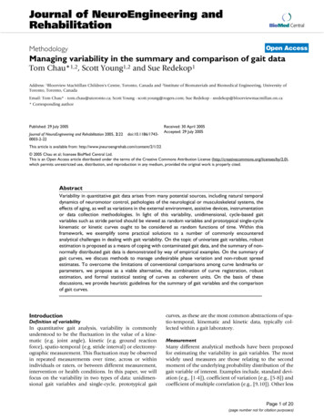
Journal of NeuroEngineering and Rehabilitation 2005, 2:22peak, which are extracted from kinematic or kinetic curveson a per cycle basis.Due to variability, univariate gait measures and parameters derived thereof should be regarded as stochasticrather than deterministic variables [47,48]. In this random variable framework, a one-dimensional gait variableis represented as X and governed by an underlying,unknown probability distribution function FX, or densitydFX. A realization of this random variabledXis written in lower case as x.function f X Inflated variability and non-robust estimationIt has been recently demonstrated that typical locationand spread estimators used in quantitative gait data analysis, i.e. mean and variance, are highly susceptible tosmall quantities of contaminant data [48]. Indeed, a fewspurious or atypical measurements can unduly inflatenon-robust estimates of gait variability. The challenge inthe summary of highly variable univariate gait data lies inreporting location and spread, faithful to the underlyingdata distribution and minimally influenced by extraordinary observations.Here, we focus on the issue of inflated variability and nonrobust estimation by examining four different spread estimators, applied to stride period data from a child withspastic diplegic cerebral palsy. As stated above, the coefficient of variation and standard deviation are routinelyemployed in the summary of gait variables. Given a sample of N observations of a gait variable X, i.e., {x1,., xN},the coefficient of variation is defined as,2NCV(X) 1/N i 1( xi - X )(1)Xwhere the numerator is simply the sample standard deviation and the denominator, X 1 / N i 1 xi , is the samNple mean. We also include two other estimators, althoughseldom used in gait analysis, to illustrate the qualitativedifferences in estimator robustness. The interquartilerange of the sample is defined asIQR(X) x0.75 - x0.25(2)where x0.75 and x0.25 are the 75% and 25% quantiles. Theq-quantile is defined as xq FX 1(q) where as usual, FX isthe probability distribution of X. Equivalently, the qquantile is the value, xq, of the random variable q f ( X)dX q . That is, q 100 percent of the randomvariable values lie below xq. We also introduce the medianabsolute deviation [49],MAD(X) med ( X - med(X) )(3)where med(X) is the median of the sample, or the 50%quantile as defined above. This last estimator is, as thename implies, the median of the absolute differencebetween the sample values and their median value. We areinterested in studying how these different estimators perform when estimating the spread in a gait variable, theobservations of which may contain outlying values orcontaminants. In the left pane of Figure 2, we show a setof stride period data recorded from a child with spasticdiplegia. The top graph shows the raw data with a numberof obvious outliers with atypically long stride times. Weadopted a common outlier definition, labeling pointsmore than 1.5 interquartile ranges away from the samplemedian as extreme values. According to this definitionthere were 21 outlying observations. In the bottom graph,the outliers have been removed. The bar graph on theright-hand side of Figure 2 portrays the spread estimatesof the stride period data, computed with each estimatorintroduced above, with and without the outliers.We note immediately that the spread estimates in thepresence of outliers are higher. The standard deviationand coefficient of variation change the most, dropping 42and 36 percent in value, respectively, upon outlierremoval. This observation is particularly important in thecomparison of gait variables, as inflated variability estimates will diminish the probability of detecting significant differences when they do in fact exist. In contrast, theinterquartile range and median absolute deviation, onlychange by 21 and 11%, respectively. We see that these latter estimates are more statistically stable, in that they arenot as greatly influenced by the presence of extremeobservations.To more fully comprehend estimator robustness or lackthereof, the field of robust statistics offers a valuable toolcalled influence functions, which as the name implies,summarizes the influence of local contaminations on estimated values. Their use in gait analysis was first introduced in the context of stride frequency estimation [48].We first introduce the concept of a functional, which canbe understood as a real-valued function on a vector spaceof probability distributions [50]. In the present context,functionals allow us to think of an estimator as a functionof a probability distribution. For example, for thePage 4 of 20(page number not for citation purposes)

Journal of NeuroEngineering and Rehabilitation 2005, gure vs.Robust2 non-robust estimators of parameter spreadRobust vs. non-robust estimators of parameter spread. The left pane shows a sequence of stride periods with outliers (top)and after removal of outliers (bottom). The right pane is a bar graph showing the values of four different spread estimatorsbefore and after outlier IQR (FX ) FX 1(0.75) FX 1(0.25) .Let the mixture distribution Fz, ε describe data governed bydistribution F but contaminated by a sample z, with probability ε. The influence function at the contamination z isdefined asIF( z) T(Fz , ) 0(4)where T(·) is the functional for the estimator of interest.The influence function for a particular estimator measuresthe incremental change in the estimator, in the presenceof large samples, due to a contamination at z. Clearly, ifthe impact of this contaminant on the estimated value isminimal, then the estimator is locally robust at z. Influence functions can be analytically derived for a variety ofcommon gait estimators (see for example, [48]), including those mentioned above. For the sake of analytical simplicity and practical convenience, we will instead usefinite sample sensitivity curves, SC(z), which can bedefined as,SC(z) (N 1){T(x1,., xN, z) - T(x1,., xN)}(5)where as above, T(·) is the functional for the estimator inquestion, and z is the contaminant observation. When N the sensitivity curve converges to the influence function for many estimators. Like the asymptotic influencefunctions, sensitivity curves describe the local impact of acontamination z on the estimator value. For the purposesof computer simulation, the functional T(x1,., xN, z) andT(x1,., xN) are simply the evaluations of the estimator ofinterest at the augmented and original samples, respectively. Figure 3 depicts the sensitivity curves for the estimators introduced in the stride period example. To generatethese curves, we used the cleansed stride period data(without outliers) and incrementally added a deviantstride period from 0.5 below the lowest sample value to0.5 above the highest sample value. The sample mean forthis data was 1.41 seconds.We observe that both standard deviation and coefficientof variation have quadratic sensitivity curves with verticesclose to the sample mean. In other words, as contaminants take on extreme low or high values, the estimatedvalues are unbounded. Clearly, these two estimators arenot robust, explaining their high sensitivity to the outliersin the stride period data. In contrast, both the interquartile range and median absolute deviation have boundedsensitivity curves, in the form of step functions. Themedian absolute deviation is actually not sensitive to contaminant values above 1.1 seconds whereas the interquartile range has a constant sensitivity to contaminant valuesover 1.6. Since most of the outliers in the stride perioddata were well above the mean, this difference explainsPage 5 of 20(page number not for citation purposes)

Journal of NeuroEngineering and Rehabilitation 2005, 5410Coefficient ofvariationB8CStandarddeviation2median ile rangeA 10.511.522.5Contaminant valueFigure 3 rideestimatorsperiod exampleof gait parameterSensitivity curves for various estimators of gait parametervariability based on the stride period example.025303540455055Range of motion of hip in sagittal plane (degrees)Figure 4 parameter distributionMultimodalMultimodal parameter distribution. Shown here is a histogram of hip range-of-motion (45 strides from 9 able-bodiedchildren) with two possible distribution functions overlaid:unimodal normal probability distribution (solid line) andbimodal gaussian mixture distribution (dashed line).the considerably lower sensitivity of the median absolutedeviation to outlier influence.From this example, we appreciate that estimators of gaitvariable spread (i.e. variability) should be selected withprudence. The popular but non-robust variability measures of standard deviation and coefficient of variationboth have 0 breakdown points [51], meaning that only asingle extreme value is required to drive the estimators toinfinity. Indeed, as seen in Figure 2, the presence of asmall fraction of outliers can unduly inflate our estimatesof gait variability. Outlier management [52], with methods such as outlier factors [53] or frequent itemsets [54],represents one possible strategy to reduce unwanted variability when using these non-robust estimators. Apartfrom the addition of a computational step, this strategyintroduces the undesirable effects of outlier smearing andmasking [55], which need to be carefully addressed.In contrast, outliers need not be explicitly identified withrobust estimation, hence circumventing the above complications and abbreviating computation. The interquartile range and median absolute deviation, havebreakdown points of 0.25 and 0.5, respectively [51]. Practically, this means that these estimators will remain stable(bounded) until the proportion of outliers reaches 25%and 50% of the sample size, respectively. To circumventexplicit outlier detection and its associated issuesaltogether, and in the presence of noisy data, which erizations of kinematic and kinetic curves, robustestimators may thus be preferable in the summary of gaitvariables.Non-gaussian distributionsEven in the absence of outliers, univariate gait data maynot adhere to a simple, unimodal gaussian distribution.In fact, distributions of gait measurements and derivedparameters may be naturally skewed, leptokurtic or multimodal [56]. Neglecting these possibilities, we may summarize gait data with location and spread values which donot reflect the underlying data distribution.Semi-parametric estimationAs an example, consider the hip range-of-motionextracted from 45 strides of 9 able-bodied children. A histogram of the data is plotted in Figure 4. Assuming thatthe data are gaussian distributed, we arrive at maximumlikelihood estimates for the mean and standard deviation,i.e. 40.4 5.1. However, the histogram clearly appears tobe bimodal. A Lilliefors test [57] confirms significantdeparture from normality (p 0.02). A number ofapproaches could be undertaken to find the underlyingmodes. One could perform simple clustering analysis[58], such as k-means clustering. Doing so reveals twowell-defined clusters, the means and standard deviationsof which are reported in Table 1. Alternatively, one couldattempt to fit to the data, a convex mixture density of theform,Page 6 of 20(page number not for citation purposes)

Journal of NeuroEngineering and Rehabilitation 2005, ble 1: Summary of bimodal ROM dataMixture distributionk-means clusteringNormal distribution37.7 2.449.1 3.50.71/0.2933.3553.8937.7 2.647.7 3.00.73/0.2732.9651.7040.4 5.130.4050.40Mode # 1Mode # 2Mixing proportion (mode I/mode 2)Critical value (lower)Critical value (upper)Stride period distribution child #1 with CPNC(6)i 1where Wi is a scalar such that i Wi 1 to preserve probability axioms, NC is the number of clusters or modes andgi ( x) 221e( x µi ) / 2σ i is a gaussian density withσ i 2πmean µi and variance σ i2 . The fitting of (6) is known assemi-parametric estimation as we do not assume a particular parametric form for the data distribution per se, butdo assume that it can modeled by a mixture of gaussians.In the present case, NC 2 and we can use a simple optimization approach to determine the parameters of themixture. In particular, we determined the parameter vector [W1, W2, µ1, σ1, µ2, σ2] to minimize the objective2nj j fˆX (x j ) N , where nj is the number of points within an interval of length around xj and N is thenumber of points in the sample. The latter term in theobjective function is a crude probability density estimate[59]. As seen in Table 1, the results of fitting this bimodalmixture yields similar results to those obtained fromclustering.functionWhat are the implications of naively summarizing thesedata with a unimodal normal distribution? First of all, theprobabilities of observing range-of-motion valuesbetween 35 and 39 degrees, where most of the observations occur, would be underestimated. Likewise, ROMvalues between 39 and 48 degrees, where the data exhibita dip in observed frequencies, would be grossly overestimated. These discrepancies are labeled as regions B and Cin Figure 4. More importantly, the discrepancies in thetails of the distributions, regions A and D, suggest that statistical comparisons with other data, say pathologicalROM, would likely yield inconsistent conclusions,depending on whether the mixture or simple distributionwas assumed. Indeed, as seen in Table 1 the lower criticalvalue of the simple normal distribution for a 5% significance level is too low. This could lead to exagerrated Type10500.511.522.53Stride period (s)Stride period distribution child #2 with CP6Number of strides Wi gi (x)fˆX ( x) Number of strides155432100.511.522.53Stride period (s)FigureComparisondrenwith5 spasticof stridediplegiaperiod distributions between 2 chilComparison of stride period distributions between 2 children with spastic diplegia. In each graph, the dashed line isthe normal probability distribution estimated for the data.The solid line is the gamma distribution fit to the data.II errors. Similarly, the upper critical value is not highenough, potentially leading to many false positive (TypeI) errors.The above example depicts bimodal data. However, themixture distribution method can be applied to arbitrarynon-normal data distributions, regardless of the underlying modality. Fitting such distributions can be accomplished by the well-established expectation-maximizationalgorithm [60]. For a comprehensive review of other semiparametric and non-parametric estimation methods, seefor example [59].Parametric estimationWhen we have some a priori knowledge about the underlying data distribution, we can adopt a simpler approachto summarize the gait data. In particular, we could fit thePage 7 of 20(page number not for citation purposes)

Journal of NeuroEngineering and Rehabilitation 2005, ble 2: Statistical comparison of stride periods under different distributional assumptionsChild12No. strides2423Gaussian distributionGamma 1710.232p 0.31data to a specific parametric form. As an example,consider the task of comparing two sets of stride perioddata from two children with spastic diplegia, with identical gross motor function classification scores [61]. Thehistograms of strides for both children are shown in Figure 5. It is known that stride period data tend to be rightskewed [56]. A careful examination of the bottom graphindicates that the histogram is indeed right-skewed. Infact, the skewness value is 1.7 and Lilliefors test for normality [57] confirms significant departure from normality(p 10-5). We thus determine the maximum likelihoodgamma distribution for these data. The gamma distribution has the following parametric form [62], 1x a 1e x / b aγ (x, a, b) b Γ(a) 0 x 0(7)otherwisewhere a is the shape parameter, b is the scale parameterand Γ(·) is the gamma function. The gamma distributionfits are plotted as solid lines in Figure 5.As in the previous example, we consider the consequenceof assuming that the data are normally distributed. Dothese two children have similar stride periods? To answerthis question, one may hastily apply a t-test, assumingthat the stride period distributions are gaussian. Theresults of this test reveal no significant differences (p 0.31), as reported in Table 2. To visualize the departurefrom normality, the maximum likelihood normal probability distribution fits to the stride data are superimposedon each histogram as a dashed curve. Note that the tails ofthe distribution are overly broad, particularly in the bottom graph. This diminishes the likelihood of detectinggenuine significant differences between the data sets.Table 2 summarizes the maximum likelihood estimates ofthe distribution parameters under the two different distributional assumptions. Under the gamma distributionassumption, the stride periods between the two childrenare statistically different (p 0.036) according to a MonteCarlo simulation of differences between 104 similarly distr

four different medical centres [13]. Dealing with variability Given the ubiquity and health relevance of variability in gait measurements, it is critical that we summarize and compare gait data in a way that reflects the true nature of their variability. Despite the apparent simplicity of these tasks, if not conducted prudently, the derived .