WIXLIB

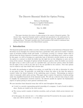
The Discrete Binomial Model for Option PricingRebecca StockbridgeProgram in Applied MathematicsUniversity of ArizonaMay 14, 2008AbstractThis paper introduces the notion of option pricing in the context of financial markets. Thediscrete time, one-period binomial model is explored and generalized to the multi-period binomial model. The multi-period model is then redeveloped using the sophisticated tools ofmartingale theory. The paper concludes with a brief extension of the results to continuous time,giving a heuristic derivation of the Black-Scholes equation.1IntroductionThe financial markets heavily utilize securities, which are abstract representations of financial value.Securities can be thought of as contracts that have a particular value, and can be traded. Commontypes of securities include stocks and bonds. A derivative security is a contract whose value isderived from the future behavior of another security (called the underlying asset), such as a stock.In this paper, we will be focusing on a particular type of derivative security known as an option.An option is a contract in which the holder has the right but not the obligation to carry out theterms of the contract. Examples of options include European options, where the holder can exercisehis right to buy (a call ) or sell (a put) at a specified date, and American options, where the holderhas the right to buy or sell at any date up to the one specified in the contract. Note that optionscan be traded at any time before their exercise date.To enable the purchasing or selling of an option, we would like to be able to determine its valueat any point in time. In particular, we would like to know the value at the time the option iscreated, before the future behavior of the underlying asset is known. Determining an option’svalue is commonly called option pricing. This paper aims to answer the question of option pricingunder the simplified framework of the binomial model. We will use a discrete-time setup in orderto simplify the mathematics involved; however, the discrete models do capture the fundamentalaspects of option pricing in more general continuous time.We now introduce basic financial terms that will be used throughout this paper: A stock is a security representing partial ownership of a company. A unit of stock is called ashare. Stocks are traded in the stock market. The money market consists of risk-free securities, such as bonds, which accrue interest overtime. In this paper, the interest rate r 0 is defined such that 1 invested in the money market attime zero will be worth (1 r) at time one.1

An arbitrage is a trading stragey that, beginning with zero wealth, has zero probability oflosing money, and has positive probability of making money. An investor can short sell a stock by borrowing it from the owner and selling it to obtain theproceeds. The investor must repurchase the stock at some point, and return the stock to theowner. If the share price falls after the investor short sells, the investor will make a profitafter repurchasing the stock. Mathematically, this is equivalent to purchasing negative sharesof stock. A portfolio is a collection of securities.In short, a stock is a risky asset whereas assets from the money market are riskless. The stock andmoney markets form the the financial world used in the models discussed below.2The Binomial ModelThe binomial model is based upon a simplification of the financial instruments involved in optionpricing, but its implications capture the essential features of more complicated continuous models.We first introduce the one-period binomial model and then discuss the more general multi-periodmodel.2.1The One-Period Binomial ModelFirst, the principal assumptions of the one-period model, in which the start of the period is calledtime zero and the end is called time one, are: A single share of stock can be subdivided for purchasing and selling; In each transaction, the price the buyer pays to purchase the stock and the amount the sellerreceives for selling the stock are the same (i.e. there are no transaction costs or fees); The interest rates for borrowing and investing are the same; The stock can take only two possible values at time one.The final condition provides this model with a binomial structure. In practice, these assumptionsare far too simplistic, but they provide a good starting point with which to begin.We consider a single stock with a price per share of S0 0 at time zero. We can imagine the priceat time one to be the result of a coin toss, either heads or tails, with probabilities p and q 1 p,respectively. (Note that p and q are not necessarily 12 .) At time one, the price per share will beeither S1 (H) or S1 (T ), with probabilities p and q.Letu S1 (H),S0d S1 (T )S0Assume that both d and u are positive, and without loss of generality, d u. The situation canthen be represented with the following diagram (see p. 1 of [4]):2

!!!!!!!S1 (H) uS0S0"""""""S1 (T ) dS0Figure 1: The one-period binomial model for t 0 and t 1.So, the financial tools available to use in this model consists of the stock described above as wellas the money market with interest rate r.A key assumption of our model is that it does not allow any arbitrage situations, as the possibilityof a riskless profit could lead to contradictory results from the model. Furthermore, any arbitragesin the real world quickly disappear as people take advantage of them. A simple condition on d andu will ensure the no-arbitrage requirement.Proposition 1The no-arbitrage assumption implies that 0 d 1 r u.ProofWe have already assumed that d 0. Now, assume that d 1 r. Then, starting with no wealthat time zero, borrow X from the money market and use that money to purchase stock. At timeone, the debt will be (1 r)X. However, if the stock price goes down, the value of the stock willbe at least (1 r)X since d 1 r. Hence, selling the stock will result in enough money to payoff the money market debt. The stock will go up with probability p 0, which will lead to a profitsince u d. Therefore, there is a positive probability of generating a riskless profit which gives anarbitrage, leading to a contradiction. So d must be less than 1 r.Similarly, assume that u 1 r. This time, short sell X of stock at time zero and invest in themoney market. At time one, the proceeds from the money market will be (1 r)X. The debt fromthe short selling will have a maximum value of uX (1 r)X, so it can be paid off. If the stockvalue decreases to dX, a profit will be made. Again there is an arbitrage and so a contradiction.Hence u 1 r.!The converse is true as well. However, the proof requires some notation that has not yet beendeveloped, so it will be presented later on in the paper.We would like to determine the value of an option at time zero. Assume that at time one, a givenoption pays an amount V1 (H) if the stock price increases and V1 (T ) if the stock price goes down.The key idea to no-arbitrage option pricing is to create a replicating portfolio through the stockand money markets (the stock in the replicating portfolio is the underlying asset of the option). By3

constructing a portfolio whose wealth at time one is equal to the value of the option, regardless ofheads or tails, we can infer that the value of the option at time zero is simply that of the replicatingportfolio. This is a direct result of the no-arbitrage assumption:Proposition 2If two portfolios give the same payoffs at all times, then they must have the same value.Note that this result applies to all types of portfolios, but for our purposes we apply it to oneportfolio consisting of an option and another consisting of single assets in the stock and moneymarkets.ProofFor illustrative purposes, consider only a one-period time frame. Assume that there exist twoporfolios, one containing Stock 1 and the other containing Stock 2, and both stocks are worth V1at time one. At time zero, Stock 1 is worth V0 and Stock 2 is worth V0! , with V0 V0! . Beginningwith no wealth, at time zero, short sell Stock 2, and purchase Stock 1. This leaves us with a totalwealth of V0! V0 . At time one, sell Stock 1, which gives exactly the amount of money needed(V1 ) to purchase Stock 2. We will then have a net wealth of V0! V0 0. Therefore, beginningwith zero wealth, we are guaranteed to make a profit, giving an arbitrage opportunity (and hencea contradiction). Extending this argument to general portfolios and multiple time-steps gives theresult above.!The previous discussion has given us the tools to determine the time zero value of an option, and wenow follow Chaper 1 of [4] to continue. Assume we have wealth X0 at time zero, and we purchase 0 shares of stock. We then have wealth X0 0 S0 that is invested in the money market at timezero. At time one, this portfolio will be worthX1 0 S1 (1 r)(X0 0 S0 ) (1 r)X0 0 (S1 (1 r)S0 ).(1)(2)Replication requires that X1 (H) V1 (H) and X1 (T ) V1 (T ), and enforcing these constraintsgives a portfolio that replicates the option’s value at time one. Rewriting Equation (2) as"1S1 (H) S0 X 0 01 r!"1X 0 0S1 (T ) S0 1 r!1V1 (H)1 r1V1 (T )1 r(3)(4)to incorporate the unknown result of the coin toss, we have a system of two linear equations withtwo unknowns, X0 and 0 . One might be tempted to solve this simple system using linear algebraictechniques, but it is more informative to proceed as follows:Multiply the first equation by a number denoted p̃ and the second by q̃ 1 p̃. Adding them gives!"11X 0 0[p̃S1 (H) q̃S1 (T )] S0 [p̃V1 (H) q̃V1 (T )] .(5)1 r1 rTo eliminate the term involving 0 , pick p̃ so that4

S0 1[p̃S1 (H) q̃S1 (T )] .1 r(6)X0 1[p̃V1 (H) q̃V1 (T )] .1 r(7)This leads to the equationSubstituting in S1 (H) uS0 and S1 (T ) dS0 , we also see thatS0 1S0[p̃uS0 (1 p̃)dS0 ] [(u d)p̃ d] .1 r1 r(8)Some rearrangement impliesp̃ 1 r d,u dq̃ u 1 r.u d(9)Solving for 0 gives us the delta-hedging formula: 0 V1 (H) V1 (T ).S1 (H) S1 (T )(10)Therefore, starting with wealth X0 and buying 0 shares of stock at time zero implies that if attime one the coin is heads, the portfolio will be worth V1 (H), and if the coin comes up tails, theportfolio will be worth V1 (T ). Hence, according to the above discussion, the option should be pricedasV0 1[p̃V1 (H) q̃V1 (T )]1 r(11)at time zero.Similar arguments to those used in the proof of Proposition 1 indicate that the value V0 given byEquation (11) is the only non-arbitrage value. This uniqueness result can be also be obtained byrecasting the pricing problem in terms of matrices. Equations (3) and (4) then become 11 1 r V1 (H) 1 1 r S1 (H) S0 X0 (12) 11 01S1 (T ) S0V1 (T )1 r1 r)* ,Ax bThis matrix equation will have a unique solution if det(A) 0.det(A) !" !"11S1 (T ) S0 S1 (H) S01 r1 r1[S1 (T ) S1 (H)]1 r5(13)(14)