Transcription
DECISION TREES: How to Construct Them and Howto Use Them for Classifying New DataAvinash KakPurdue UniversityNovember 20, 202011:29amAn RVL Tutorial Presentation(First presented in Fall 2010; Updated in November 2020) 2020 Avinash Kak, Purdue University
Decision TreesAn RVL Tutorial by Avi KakCONTENTSPage1Introduction32Entropy83Conditional Entropy134Average Entropy155Using Class Entropy to Discover the Best Featurefor Discriminating Between the Classes176Constructing a Decision Tree217Incorporating Numeric Features308The Python Module399The Perl 434410 Bulk Classification of Test Data in CSV Files4911 Dealing with Large Dynamic-Range andHeavy-tailed Features5112 Testing the Quality of the Training Data5313 Decision Tree Introspection5814 Incorporating Bagging6415 Incorporating Boosting7016 Working with Randomized Decision Trees7717 Speeding Up DT Based Classification With Hash Tables8318 Constructing Regression Trees8919 Historical Antecedents of Decision TreeClassification in Purdue RVL932
Decision TreesAn RVL Tutorial by Avi KakBack to TOC1:Introduction Let’s say your problem involves making a decision based on Npieces of information. Let’s further say that you can organizethe N pieces of information and the corresponding decision asfollows:f 1f 2f 3.f N ----------------------------val 1val 1val 1val 1val 1.val 2val 2val 2val 2val 2val 3val 3val 3val 3val 3.val Nval Nval Nval Nval N d1d2d1d1d3Such data is commonly referred to as structured or tabulateddata, the sort of data that you can extract from a spreadsheet.[My DecisionTree module assumes that this type of data has been exported from a database inthe form of a CSV file.] For convenience, we think of each column of the data tabulatedas shown above as representing a feature f i whose value goesinto your decision making process. Each row of the tablerepresents a set of values for all the features and thecorresponding decision.3
Decision TreesAn RVL Tutorial by Avi Kak As to what specifically the features f i shown above would be,that would obviously depend on your application. [In a medical context,each feature f i could represent a laboratory test on a patient, the value val i the result of the test, and thedecision d i the diagnosis. In drug discovery, each feature f i could represent the name of an ingredient inthe drug, the value val i the proportion of that ingredient, and the decision d i the effectiveness of the drugin a drug trial. In a Wall Street sort of an application, each feature could represent a criterion (such as the]price-to-earnings ratio) for making a buy/sell investment decision, and so on. If the different rows of the training data, arranged in the form ofa table shown on the previous page, capture adequately thestatistical variability of the feature values as they occur in thereal world, you may be able to use a decision tree for automatingthe decision making process on any new data. [As to what I mean by“capturing adequately the statistical variability of feature values”, see Section 12 of this tutorial.] Let’s say that your new data record for which you need to makea decision looks like:new val 1new val 2new val 2.new val Nthe decision tree will spit out the best possible decision to makefor this new data record given the statistical distribution of thefeature values for all the decisions in the training data suppliedthrough the table on page 3. The “quality” of this decisionwould obviously depend on the quality of the training data, asexplained in Section 12.4
Decision TreesAn RVL Tutorial by Avi Kak This tutorial will demonstrate how the notion of entropy can beused to construct a decision tree in which the feature tests formaking a decision on a new data record are organized optimallyin the form of a tree of decision nodes. In the decision tree that is constructed from your training data,the feature test that is selected for the root node causesmaximal disambiguation of the different possible decisions for anew data record. [In terms of information content as measured by entropy, the feature test atthe root would cause maximum reduction in the decision entropy in going from all the training data taken]together to the data as partitioned by the feature test. One then drops from the root node a set of child nodes, one foreach value of the feature tested at the root node for the case ofsymbolic features. For the case when a numeric feature is testedat the root node, one drops from the root node two child nodes,one for the case when the value of the feature tested at the rootis less than the decision threshold chosen at the root and theother for the opposite case. Subsequently, at each child node, you pose the same questionyou posed at the root node when you selected the best featureto test at that node: Which feature test at the child node inquestion would maximally disambiguate the decisions for thetraining data associated with the child node in question?5
Decision TreesAn RVL Tutorial by Avi Kak In the rest of this Introduction, let’s see how a decision-treebased classifier can be used by a computer vision system toautomatically figure out which features work the best in orderto distinguish between a set of objects. We assume that thevision system has been supplied with a very large number ofelementary features (we could refer to these as the vocabulary ofa computer vision system) and how to extract them fromimages. But the vision system has NOT been told in advance asto which of these elementary features are relevant to the objects. Here is how we could create such a self-learning computer visionsystem:– We show a number of different objects to a sensor system consistingof cameras, 3D vision sensors (such as the Microsoft Kinect sensor),and so on. Let’s say these objects belong to M different classes.– For each object shown, all that we tell the computer is its classlabel. We do NOT tell the computer how to discriminate betweenthe objects belonging to the different classes.– We supply a large vocabulary of features to the computer and alsoprovide the computer with tools to extract these features from thesensory information collected from each object.– For image data, these features could be color and texture attributesand the presence or absence of shape primitives. [For depth data, thefeatures could be different types of curvatures of the object surfaces and junctions formed by the joinsbetween the surfaces, etc.]6
Decision TreesAn RVL Tutorial by Avi Kak– The job given to the computer: From the data thus collected, itmust figure out on its own how to best discriminate between theobjects belonging to the different classes. [That is, the computer must learn on itsown what features to use for discriminating between the classes and what features to ignore.] What we have described above constitutes an exercise in aself-learning computer vision system. As mentioned in Section 19 of this tutorial, such a computervision system was successfully constructed and tested in mylaboratory at Purdue as a part of a Ph.D thesis. This work isdescribed in the following lications/Grewe95Interactive.pdf7
Decision TreesAn RVL Tutorial by Avi KakBack to TOC2:Entropy Entropy is a powerful tool that can be used by a computer todetermine on its own own as to what features to use and how tocarve up the feature space for achieving the best possiblediscrimination between the classes. [You can think of each decision of a certaintype in the last column of the table on page 3 as defining a class. If, in the context of computer vision, all theentries in the last column boil down to one of “apple,” “orange,” and “pear,” then your training data has a]total of three classes. What is entropy? Entropy is fundamentally a numeric measure of the overalluncertainty associated with a random quantity. If a random variable X can take N different values, the ithvalue xi with probability p(xi), we can associate the followingentropy with X:H(X) NXi 18p(xi) log2 p(xi)
Decision TreesAn RVL Tutorial by Avi Kak To gain some insight into what H measures, consider the casewhen the normalized histogram of the values taken by therandom variable X looks like1/8 hist(X) (normalized) -------------------------------------------- 12345678 In this case, X takes one of 8 possible values, each with aprobability of p(xi) 1/8. For a such a random variable, theentropy is given byH(X) 8X1log28X1log2 2 3i 1 i 1 88183 bits Now consider the following example in which the uniformlydistributed random variable X takes one of 64 possible values:9
Decision TreesAn RVL Tutorial by Avi Kak1/64histogram (normalized) . ------------------------------------------------- 1234.6364 In this case,H(X)64X11log2 6464i 1 8X1i 1 8log2 2 66 bits So we see that the entropy, measured in bits because of 2 beingthe base of the logarithm, has increased because now we havegreater uncertainty or “chaos” in the values of X. It can nowtake one of 64 values with equal probability. Let’s now consider an example at the other end of the “chaos”:We will consider an X that is always known to take on aparticular value:10
Decision TreesAn RVL Tutorial by Avi Kak1.0 histogram (normalized) 0 0 0 0 . 0 0 ------------------------------------------------- 123.k.6364 In this case, we obviously havep(xi) 10xi kotherwise The entropy for such an X would be given by:H(X) NXp(xi) log2 p(xi)i 1 [p1 log2 p1 .pk log2 pk . pN log2 pN ] 1 log2 1 bits 0 bitswhere we use the fact that as p 0 , p log p 0 in all ofthe terms of the summation except when i k.11
Decision TreesAn RVL Tutorial by Avi Kak So we see that the entropy becomes zero when X has zero chaos. In general, the more nonuniform the probabilitydistribution for an entity, the smaller the entropyassociated with the entity.12
Decision TreesAn RVL Tutorial by Avi KakBack to TOC3:Conditional Entropy Given two interdependent random variables X and Y , theconditional entropy H(Y X) measures how much entropy(chaos) remains in Y if we already know the value of therandom variable X. In general,H(Y X) H(X, Y ) H(X)The entropy contained in both variables when taken together isH(X, Y ). The above definition says that, if X and Y areinterdependent, and if we know X, we can reduce our measureof chaos in Y by the chaos that is attributable to X. [For independentX and Y , one can easily show that H(X, Y ) H(X) H(Y ).] But what do we mean by knowing X in the context of X and Ybeing interdependent? Before we answer this question, let’s firstlook at the formula for the joint entropy H(X, Y ), which isgiven byH(X, Y ) Xi,j13 p xi, yj log2 p xi, yj
Decision TreesAn RVL Tutorial by Avi Kak When we say we know X, in general what we mean is that weknow that the variable X has taken on a particular value. Let’ssay that X has taken on a specific value a. The entropyassociated with Y would now be given by: H Y X a Xi p yi X a log2 p yi X a The formula shown for H(Y X) on the previous page is theaverage of H Y X a over all possible instantiations a for X,as I’ll show in the next section.14
Decision TreesAn RVL Tutorial by Avi KakBack to TOC4:Average Entropies Given N independent random variables X1 , X2, . . . XN , we canassociate an average entropy with all N variables byHav NXH(Xi ) p(Xi)1 For another kind of an average, the conditional entropyH(Y X) is also an average, in the sense that the right hand sideshown below is an average with respect to all of the differentways the conditioning variable can be instantiated:H Y X Xa H Y X a p X a) where H Y X a is given by the formula at the bottom of theprevious page. To establish the claim made above, note that15
Decision TreesAn RVL Tutorial by Avi Kak X H Y X a p(X a)H Y Xa o XnX p(X a)p yj X a log2 p yj X aaj XX p yj xi log2 p yj xi p(xi )i X X p(xi , yj )i jjXXilog2p(xi )p(xi , yj )p(xi )p(xi )hip(xi , yj ) log2 p(xi , yj ) log2 p(xi )j H(X, Y ) XX H(X, Y ) Xip(xi , yj ) log2 p(xi )jp(xi ) log2 p(xi )i H(X, Y ) H(X)In the above derivation, the 3rd expression is a rewrite of the 2ndwith a more compact notation. [In the 7 , we note that we get a marginalprobability when a joint probability is summed with respect to its free variable.]th16
Decision TreesAn RVL Tutorial by Avi KakBack to TOC5:Using Class Entropy to Discover the BestFeature for Discriminating Between theClasses Consider the following question: Let us say that we are giventhe measurement data as described at the beginning of Section1. Let the exhaustive set of features known to the computer be{f1, f2 , ., fK }. Now the computer wants to know as to which of these featuresis best in the sense of being the most class discriminative. How does the computer do that? To discover the best feature, all that the computer has to do isto compute the class entropy as conditioned on each specificfeature f separately as follows:H(C f ) X H C v(f ) a p v(f ) aawhere the notation v(f ) a means that the value of feature fis some specific value a. The computer selects that feature f forwhich H(C f ) is the smallest value. [In the formula shown above, the averaging17
Decision TreesAn RVL Tutorial by Avi Kak]carried out over the values of the feature f is the same type of averaging as shown at the bottom of page 15.NOTATION:Note that C is a random variable over the class labels. If your training datamentions the following three classes: “apple,” “orange,” and “pear,” then C as a random variable takes one ofthese labels as its value. Let’s now focus on the calculation of the right hand side in theequation shown above. The entropy in each term on the right hand side in the equationshown on the previous page can be calculated by H C v(f ) a X p Cm v(f ) a log2 p Cm v(f ) amwhere Cm is the name of the mth class and the summation isover all the classes. But how do we figure out p Cm v(f ) a that is needed onthe right hand side? Wetwo different ways for calculating will next presentp Cm v(f ) a . The first approach works if we can assumethat the objects shown to the sensor system are drawnuniformly from the different classes. If that is not the case, onemust use the second approach.18
Decision TreesAn RVL Tutorial by Avi Kak Our first approach for calculating p(Cm v(f ) a) is count-based:Given M classes of objects that we show to a sensor system, we pick objects randomly from thepopulation of all objects belonging to all classes. Say the sensor system is allowed to measure Kdifferent kinds of features: f1 , f2 , ., fK . For each feature fk , the sensor system keeps a count of thenumber of objects that gave rise to the v(fk ) a value. Now we estimate p(Cm v(f ) a) for anychoice of f fk simply by counting off the number of objects from class Cm that exhibited thev(fk ) a measurement. Our second approach for estimating p Cm v(f ) a uses the Bayes’ Theorem: p Cm v(f ) a p v(f ) a Cm p(Cm) p v(f ) aThis formula also allows us to carry out separate measurementexperiments for objects belonging to different classes. Another advantage of the above formula is that it is no longer aproblem if only a small number of objects are available for someof the classes — such non-uniformities in object populations aretaken care of by the p(Cm) term. The denominator in the formula shown above can be taken careof by the required normalization: X p Cm v(f ) am19 1
Decision TreesAn RVL Tutorial by Avi Kak What’s interesting is that if we do obtain p v(f ) a through the normalization mentioned above, we can also use it in theformula for calculating H(C f ) as shown on page 17.Otherwise, p v(f ) a would need to be estimated directlyfrom the raw experimental data. So now we have all the information that is needed to estimatethe class entropy H(C f ) for any given feature f by using theformula shown on page 17. It follows from the nature of entropy (See Section 2) that thesmaller the value for H(C f ), especially in relation to the valueof H(C), the greater the class discriminatory power of f . Should it happen that H(C f ) 0 for some feature f , thatimplies that feature f can be used to identify objects belongingto at least one of the M classes with 100% accuracy.20
Decision TreesAn RVL Tutorial by Avi KakBack to TOC6:Constructing a Decision Tree Now that you know how to use the class entropy to find thebest feature that will discriminate between the classes, we willnow extend this idea and show how you can construct a decisiontree. Subsequently the tree may be used to classify futuresamples of data. But what is a decision tree? For those not familiar with decision tree ideas, the traditionalway to classify multidimensional data is to start with a featurespace whose dimensionality is the same as that of the data. In the traditional approach, each feature in the space wouldcorrespond to the attribute that each dimension of the datameasures. You then use the training data to carve up thefeature space into different regions, each corresponding to adifferent class. Subsequently, when you are trying to classify anew data sample, you locate it in the feature space and find theclass label of the region to which it belongs. One can also givethe data point the same class label as that of the nearesttraining sample. (This is referred to as the nearest neighbor21
Decision TreesAn RVL Tutorial by Avi Kakclassification.) A decision tree classifier works differently. When you construct a decision tree, you select for the root nodea feature test that can be expected to maximally disambiguatethe class labels that could be associated with the data you aretrying to classify. You then attach to the root node a set of child nodes, one foreach value of the feature you chose at the root node. [This statementis not entirely accurate. As you will see later, for the case of symbolic features, you create child nodes for onlythose feature values (for the feature chosen at the root node) that reduce the class entropy in relation to the] Now at each child node you pose thesame question that you posed when you found the best featureto use at the root node: What feature at the child node inquestion would maximally disambiguate the class labels to beassociated with a given data vector assuming that the datavector passed the root node on the branch that corresponds tothe child node in question. The feature that is best at each nodeis the one that causes the maximal reduction in class entropy atthat node.value of the class entropy at the root. Based on the discussion in the previous section, you alreadyknow how to find the best feature at the root node of a decision22
Decision TreesAn RVL Tutorial by Avi Kaktree. Now the question is: How we do construct the rest of thedecision tree? What we obviously need is a child node for every possible valueof the feature test that was selected at the root node of the tree. Assume that the feature selected at the root node is fj and thatwe are now at one of the child nodes hanging from the root. Sothe question now is how do we select the best feature to use atthe child node. The root node feature was selected as that f which minimizedH(C f ). With this choice, we ended up with the feature fj atthe root. The feature to use at the child on the branchv(fj ) aj will be selectedas that f 6 fj which minimizes H C v(fj ) aj , f . [REMINDER: Whereas v(fj ) stands forthe “value of feature fj ,” the notation aj stands for a specificvalue taken by that feature.] That is, for any feature f not previously used at the root, wefind the conditional entropy (with respect to our choice for f ) when weare on the v(fj ) aj branch:23
Decision TreesAn RVL Tutorial by Avi Kak H C f, v(fj ) ajX H C v(f ) b, v(fj ) aj p v(f ) b, v(fj ) ajbWhichever feature f yields the smallest value for the entropymentioned on the left hand side of the above equation willbecome the feature test of choice at the branch in question. Strictly speaking, the entropy formula shown above for thecalculation of average entropy is not correct since it does notreflect the fact that the probabilistic averaging on the right handside is only with respect to the values taken on by the feature f . In the equation shown above, for the summation shown on theright to yield a true average with respect to different possiblevalues for the feature f , the formula would need to be expressedas1 H C f, v(fj ) aj p v(f ) b, v(fj ) ajX H C v(f ) b, v(fj ) aj P baj p v(f ) b, v(fj ) aj1 In my lab at Purdue, we refer to such normalizations in the calculation of average entropy as “JZ Normalization”—after Padmini Jaikumar and Josh Zapf.24
Decision TreesAn RVL Tutorial by Avi Kak The component entropies in the summation on the right in theprevious equation are given by H C v(f ) b, v(fj ) aj X p Cm v(f ) b, v(fj ) aj log2 p Cm v(f ) b, v(fj ) aj mfor any given feature f 6 fj . The conditional probability needed above can be estimatedusing Bayes Theorem: p Cm v(f ) b, v(fj ) aj p v(f ) b, v(fj ) aj Cm p Cm p v(f ) b, v(fj ) aj p v(f ) b Cm p v(fj ) aj Cm p Cm p v(f ) b p v(fj ) ajwhere the second equality is based on the assumption that thefeatures are statistically independent.25
Decision TreesAn RVL Tutorial by Avi KakFeature Tested at Rootff 1jFeature Tested at This Nodefkjf 2jFeature Tested at This Nodefl You will add other child nodes to the root in the same manner,with one child node for each value that can be taken by thefeature fj . This process can be continued to extend the tree further toresult in a structure that will look like what is shown in thefigure above. Now we will address the very important issue of the stoppingrule for growing the tree. That is, when does a node get afeature test so that it can be split further and when does it not? A node is assigned the entropy that resulted in its creation. Forexample, the root gets the entropy H(C) computed from theclass priors.26
Decision TreesAn RVL Tutorial by Avi Kak The children of the root are assigned the entropy H(C fj ) thatresulted in their creation. A child node of the root that is on the branch v(fj ) aj gets itsown feature test (and is split further) if and only if we can finda feature fk such that H C fk , v(fj ) aj is less than the entropyH(C fj ) inherited by the child from the root. If the condition H C f, v(fj ) aj H C fj ) cannot besatisfied at the child node on the branch v(fj ) aj of the rootfor any feature f 6 fj , the child node remains without a featuretest and becomes a leaf node of the decision tree. Another reason for a node to become a leaf node is that we haveused up all the features along that branch up to that node. That brings us to the last important issue related to theconstruction of a decision tree: associating class probabilitieswith each node of the tree. As to why we need to associate class probabilities with thenodes in the decision tree, let us say we are given forclassification a new data vector consisting of features and theircorresponding values.27
Decision TreesAn RVL Tutorial by Avi Kak For the classification of the new data vector mentioned above,we will first subject this data vector to the feature test at theroot. We will then take the branch that corresponds to thevalue in the data vector for the root feature. Next, we will subject the data vector to the feature test at thechild node on that branch. We will continue this process untilwe have used up all the feature values in the data vector. Thatshould put us at one of the nodes, possibly a leaf node. Now we wish to know what the residual class probabilities areat that node. These class probabilities will represent ourclassification of the new data vector. If the feature tests along a path to a node in the tree arev(fj ) aj , v(fk ) bk , . . ., we will associate the following classprobability with the node: p Cm v(fj ) aj , v(fk ) bk , . . .for m 1, 2, . . . , M where M is the number of classes. The above probability may be estimated with Bayes Theorem:28
Decision TreesAn RVL Tutorial by Avi Kak p Cm v(fj ) aj , v(fk ) bk , . . . p v(fj ) aj , v(fk ) bk , . . . Cm p Cm p v(fj ) aj , v(fk ) bk , . . . If we again use the notion of statistical independence betweenthe features both when they are considered on their own andwhen considered conditioned on a given class, we can write: p v(fj ) aj , v(fk ) bk , . . . Y p v(f ) valueY p v(f ) value Cmf on branch p v(fj ) aj , v(fk ) bk , . . . Cm f on branch29
Decision TreesAn RVL Tutorial by Avi KakBack to TOC7:Incorporating Numeric Features A feature is numeric if it can take any floating-point value froma continuum of values. The sort of reasoning we have describedso far for choosing the best feature at a node and constructing adecision tree cannot be applied directly to the case of numericfeatures. However, numeric features lend themselves to recursivepartitioning that eventually results in the same sort of adecision tree you have seen so far. When we talked about symbolic features in Section 5, wecalculated the class entropy with respect to a feature byconstructing a probabilistic average of the class entropies withrespect to knowing each value separately for the feature. Let’s say f is a numeric feature. For a numeric feature, a betterapproach consists of calculating the class entropy vis-a-vis adecision threshold on the feature values:30
Decision TreesAn RVL Tutorial by Avi Kak H C vth(f ) θ H C v(f ) θ p v(f ) θ H C v(f ) θ p v(f ) θwhere vth (f ) θ means that we have set the decision thresholdfor the values of the feature f at θ for the purpose ofpartitioning the data into parts, one for which v(f ) θ andthe other for which v(f ) θ. The left side in the equation shown above is the average entropyfor the two parts considered separately on the right hand side.The threshold for which this average entropy is the minimum isthe best threshold to use for the numeric feature f . To illustrate the usefulness of minimizing this average entropyfor discovering the best threshold, consider the case when wehave only two classes, one for which all values of f are less thanθ and the other for which all values of f are greater than θ. Forthis case, the left hand side above would be zero. The components entropies on the right hand side in theprevious equation can be calculated by H C v(f ) θ X p Cm v(f ) θ log2 p Cm v(f ) θ mand31
Decision TreesAn RVL Tutorial by Avi Kak H C v(f ) θ X p Cm v(f ) θ log2 p Cm v(f ) θ m We can estimatep Cm v(f ) θ andp Cm v(f ) θ by using the Bayes’Theorem: p Cm v(f ) θ p v(f ) θ Cm p(Cm) p v(f ) θ p Cm v(f ) θ p v(f ) θ Cm p(Cm) p v(f ) θand The various terms on the right sides in the two equationsshown above can be estimated directly from the training data. However, in practice, you are better off using the normalizationshown on the next page for estimating the denominator in theequations shown above. Although the denominator in the equations shown above can beestimated directly from the training data, you are likely toachieve superior results if you calculate this denominatordirectly from (or, at least, adjust its calculated value with) the32
Decision TreesAn RVL Tutorial by Avi Kakfollowing normalization constraint on the probabilities on theleft:X p Cmv(f ) θ 1v(f ) θ 1mandX p Cmm Now we are all set to use this partitioning logic to choose thebest feature for the root node of our decision tree. We proceedas follows. Given a set of numeric features and a training data file, we seekthat numeric feature for which the average entropy over the twoparts created by the thresholding partition is the least. For each numeric feature, we scan through all possiblepartitioning points (these would obviously be the samplingpoints over the interval corresponding to the values taken bythat feature), and we choose that partitioning point whichminimizes the average entropy of the two parts. We considerthis partitioning point as the best decision threshold to usevis-a-vis that feature.33
Decision TreesAn RVL Tutorial by Avi Kak Given a set of numeric features, their associated best decisionthresholds, and the corresponding average entropies over thepartitions obtained, we select for our best feature that featurethat has the least average entropy associated with it at its bestdecision threshold. After finding the best feature for the root node in the mannerdescribed above, we can drop two branches from it, one for thetraining samples for which v(f ) θ and the other for thesamples for which v(f ) θ as shown in the figure below:Feature Tested at Rootfv( f ) θjjv( f ) θj The argument stated above can obviously be extended to amixture of numeric and symbolic features. Given a mixture orsymbolic and numeric features, we associate with each symbolicfeature the best possible entropy calculated in the mannerexplained in Section 5. And, we associate with each numericfeature the best entropy that corresponds to the best thresholdchoice for that feature. Given all the features and their34
Decision TreesAn RVL Tutorial by Avi Kakassociated best class entropies, we choose that feature for theroot node of our decision tree for which the class entropy is theminimum. Now that you know how to construct the root node for the casewhen yo
new data record. [In terms of information content as measured by entropy, the feature test at the root would cause maximum reduction in the decision entropy in going from all the training data taken together to the data as partitioned by the feature test.] One then drops from the root node a set of child nodes, one for