WIXLIB

International Journal of Academic Research in Accounting, Finance and Management SciencesVol. 3 (3), pp. 78–88, 2013 HRMARS2. The Model of TOC-SCRSFigure 3 shows the basic concept of TOC-SCRS. This mechanism explains the replenishment mechanismthat each sale point (namely plant, warehouse, or retailer) in the supply chain must be applied to (Cole andJacob, 2002; Wu et al., 2010; Wu et al., 2011), and under the circumstances that sales of each period (thedaily or weekly sales of a sale point or the sum of total demand or total purchase from the downstreamcompanies) is determined, such mechanism contains three kinds of parameters, they are respectively thereplenishment time, maximum inventory level, and replenishment quantity, details are described in thefollowing:Demand ofdownstreamReplenishment timeDemand(TRR FR RRT)DemandCentralwarehouseDemandDemand ofdownstreamDemand ofdownstreamRegionalDemandWarehouseBuffer LevelDemand ofdownstreamMa xi mum demand of ea ch phase (D)TRR(ri) Time to Reliably Replenish for product i.; RRT(li) Reliable Replenishment Time for product i.FR(fi) Frequency of Replenishment (FR) for product i.Figure 3.The replenishment mechanism of TOC-SCRS (Cole and Jacob, 2002)(1) Replenishment time: The sum of replenishment frequency and the lead time it requires.。Replenishment frequency is the how long to replenish once, which is the time interval from theprevious replenishment order to the current replenishment order.。Replenishment lead time: How long does it take from replenishment order is released until productsare delivered to the destination, and such time may include the production time the upstream companiesneed, or the delivery time between downstream companies and the sale point, etc.(2) Maximum inventory level: The maximum inventory quantity within consecutive replenishment timeis estimated in accordance with the length of replenishment time based on the record of the previous sales.For example, if the replenishment time is 3 days, and the maximum value of the consecutive 3-day salesaccording to the previous sales record is defined as the maximum inventory quantity of the sale point. Inother words, the maximum inventory quantity is determined in accordance with the replenishment time andprevious sales, therefore the relationship can be presented in the following formula (1), and the detailedformula and application example will be shown in Figure 4.Maximum inventory quantity f (replenishment time, sales of each phase)(1)81

International Journal of Academic Research in Accounting, Finance and Management SciencesVol. 3 (3), pp. 78–88, 2013 HRMARSFigure 4.The Model of Buffer Level(3) Replenishment quantity: The volume of each replenishment order is the total sales of the sale pointfrom the previous replenishment order to the current replenishment order, namely to replenish how much isused, for example, if the replenishment frequency is once in two days, and then the replenishment quantity isthe sales of the recent two days. In other words, the replenishment quantity is determined by thereplenishment frequency and the sales within the period, therefore the relationship can be presented in thefollowing formula (4), and the detailed formula and application example will be shown in Figure 5.Replenishment quantity f (replenishment frequency, sales of each phase)82(4)

International Journal of Academic Research in Accounting, Finance and Management SciencesVol. 3 (3), pp. 78–88, 2013 HRMARSFigure 5. The Model of Replenishment QuantityAmong the above three parameters, the replenishment time and replenishment frequency must bedetermined in accordance with needs by the user, but TOC stresses that unless environmental and technicalconstraints are found, such as sailing schedule or route change, otherwise the shorter the replenishmentfrequency the better the performance (like one day). As for the maximum inventory level and replenishmentquantity, are determined by the known demand of each phase and replenishment time (frequency).Secondly, in terms of impacts caused by unexpected situations, the TOC-SCRS couples with the BMmechanism system. The BM is basically an inventory monitoring mechanism that is applied to each sale point,mainly aiming at monitoring the impacts caused by unexpected situations in the supply chain, such as thedelay of trucks or sudden increase in sales, etc, for it is as well an estimation method for evaluating the level83

International Journal of Academic Research in Accounting, Finance and Management SciencesVol. 3 (3), pp. 78–88, 2013 HRMARSof impact. Its concept of application is similar to the buffer management mechanism collocated with theproduction management and drum-buffer-rope (DBR) (Schragenheim and Ronen, 1991). However, the buffermanagement mechanism that goes along with the DBR is the buffer time, but over here what the buffermanagement mechanism monitors in terms of inventory is the inventory quantity. A buffer managementmechanism of monitoring is needed for each commodity and the size of the largest buffer (inventory) is themaximum inventory level, the three areas represent the three inventory monitoring areas, derived from themaximum inventory level division, and they are respectively the action, warning, and safe areas. When theinventory is more than 2/3 (inclusive) of buffer, it means the stock is abundant, for we do not need to payattention, thus such area is called the safe area; when the inventory is more than 1/3 (inclusive) or less than2/3 of buffer, it means the stock is not very abundant, for it is not up to the state of shortage, hence we onlyneed to be alerted and pay attention to the subsequent changes, no actions are needed to be done so far,hence this area is called the warning area; when the inventory is consumed fully and less than 1/3 of buffer, itmeans it may be out of stock at any time, so we must immediately request an emergency replenishment fromupstream companies, hence this area is called the action area. Through the buffer management monitoringmechanism of inventory, unexpected situations or variations that may cause a shortage can be avoided.3. Characteristics and Problems of the TOC-SCRSAccording to the above descriptions, the TOC-SCRS basically contains the following characteristics:(1) In general, according to the inventory theory, the inventory mechanism is divided into successive(or quantitative) replenishment, such as (s, S), and fixed period replenishment, such as (R, S) (Silver et al.,1998), and so, the TOC-SCRS is considered as a fixed period replenishment method.(2) The determination of TOC-SCRS replenishment quantity and maximum inventory level varies fromthe general fixed period replenishment method. The general fixed period replenishment methods, such as (R,S) or (R, Q), the replenishment quantity (Q) and the maximum inventory level (S) are determined by EconomicOrder Quantity (EOQ), Q EOQ or S s EOQ (Silver et al., 1998). Therefore, the replenishment frequency andthe length of replenishment time have no direct impacts on the replenishment quantity or the maximuminventory level. As for the replenishment quantity of TOC-SCRS, it is determined by the replenishmentfrequency and the sales between two replenishment periods, it is similar to Lot-for-Lot (L4L) of materialrequirement planning (MRP), hence the shorter the replenishment frequency, the smaller the replenishmentquantity. And the maximum inventory level is determined by the replenishment time and sales within suchtime, hence the shorter the replenishment time, the smaller the maximum inventory level. In other words,the length of replenishment frequency and replenishment time is the key factor to determine thereplenishment quantity and the maximum inventory level of TOC-SCRS. This point (how it determines thereplenishment quantity and the maximum inventory level) shows the biggest difference in the TOC -SCRScompared to general fixed period replenishment mechanisms.(3) Because the replenishment quantity and the maximum inventory level of TOC-SCRS are determinedby the replenishment frequency and replenishment lead time; therefore, how managers control the inventorylevel and make adjustments in accordance with changes in sales is more direct and more efficient. And as longas we can improve the replenishment frequency and replenishment time, the inventory level can thus bereduced, and most importantly, we may avoid shortages caused by lower inventories. This is one of thereasons why the TOC-SCRS is widely accepted by practitioners.(4) Will the number and cost of delivery increase followed by the reduction in the replenishmentquantity? According to the actual case report (Kendall, 2006), there will not be any increases. A delivery of 10commodities, 50 of each (three-month supply) and a delivery of 50 commodities, 10 of each (three-weeksupply), both shares the same delivery frequency, hence no extra delivery frequency or cost will be occurred.Due to the key determinant of the replenishment quantity and the maximum inventory level of TOCSCRS lies in the length of replenishment frequency and replenishment time, and such characteristic (how itdetermines the replenishment quantity and the maximum inventory level) explains how the TOC-SCRS variesfrom general replenishment mechanism, therefore we will be looking at the impacts on the inventory causedby different replenishment frequency and replenishment time.84

International Journal of Academic Research in Accounting, Finance and Management SciencesVol. 3 (3), pp. 78–88, 2013 HRMARS4. Impacts on the inventory in terms of different replenishment time4.1. Impacts on the Buffer Level in terms of the size of TRRAccording to the TOC, the buffer level is the biggest demand within the TRR. Take the past 24-day salesof Product A shown in Table 1 as example, when the TRR 4, we can then find out the successive sales of theprevious 4 days starting from the fourth day, and so, there is a total of 21 values; and we may obtain themaximum, Buffera Max｛(32 36 35 22), (36 26) , (32 31)｝ 127. When the TRR 8, theinventory level is to be calculated starting from the eighth day and we may obtain the maximum of sales ofsuccessive 8 days, Buffera Max｛(32 36 27) , , (36 35)｝ 242, the daily successive buffercalculation is as shown in Table 1, and we can find that the demand of each phase and the length of TRRdetermine the Buffer Level.Table 1. The inventory buffer in terms of different TRR aPeriod (day)Sales quantitySuccessive 4-day salesSuccessive 8-day salesPeriod (day)Sales quantitySuccessive 4-day salesSuccessive 8-day 72404.2 Impacts on the inventory in terms of different replenishment frequency and replenishment lead timeBecause the purchase quantity is generated within the length of each replenishment frequency time,therefore Qi,j is as the demand of each order period and FRi is the factor that determines the purchasequantity; as for the replenishment quantity is generated within the length of each replenishment lead time forRi,j is as the purchase quantity, therefore RRTi is the factor that determines the purchase timing. The time toreliably replenishment (TRR) is composed of the frequency of replenishment (FR) and reliable replenishmenttime (RRT), so let’s use TRR 8 as example, as the maximum FR is FR TRR - 1 and the minimum is FR 1, howdoes it affect the inventory. Take the demand of successive 20-day shown in Tables 2 and 3 as example, whenFR 1, RRT 7, and FR 7, RRT 1, the ending inventories shown on Tables 2 and 3 are very different, andfurther discussions will continue in the next section.Table 2. Changes in the inventory when FR 1, RRT 7Period (day)1 2 3Demand quantity 23 33 29Order quantity23 33 29Purchase quantityEnding inventory 355 322 2934 5 6 7 835 38 28 38 3735 38 28 38 3723258 220 192 154 6183333311641927272716420262638176Table 3. Changes in the inventory when FR 7, RRT 1Period (day)1 2 3 4 5 6Demand quantity 23 33 29 35 38 28Order quantityPurchase quantityEnding inventory 355 322 293 258 220 1927 8 9 10 11 12 1338 37 28 31 31 27 38224224154 341 313 282 251 224 18614 15 16 17 18 19 2027 27 26 36 33 27 26219219159 351 325 289 256 229 20385

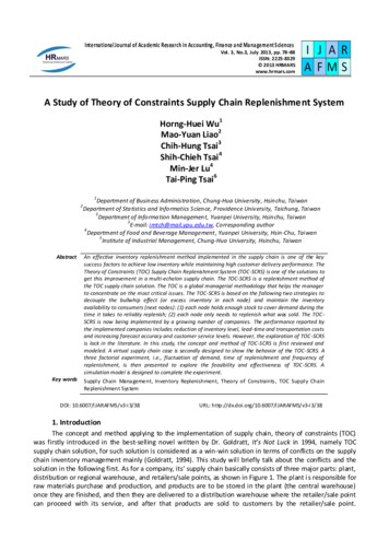
International Journal of Academic Research in Accounting, Finance and Management SciencesVol. 3 (3), pp. 78–88, 2013 HRMARS5. Experimental design and analytical results5.1. Environment and parameter settingsBecause main factors that can affect the inventory level contain the average daily demand, demandstandard deviation, and TRR, therefore this study has established 36 combinations by using high, medium, lowaverage daily demands; high, medium, low demand standard deviations, long, short TRR values, and long,short FR values, etc. According to different combination of factors based on different levels, take a certainproduct as example, the average daily demands are 100, 300, and 500, demand standard deviations are 5%,10%, and 20%, the TRR values are 5 and 10, and FR and RRT are 1, 4 and 1, 9 days respectively, as shown inTable 4. This experiment used the EXCEL software for stimulation, the average daily demand was normallydistributed, and the initial Buffer rate was known; the 3 3 2 2 36 of experiments were implemented byusing different factor parameters, and a 200-day experimentation was applied to each group of parameters inorder to obtain the representative data. At the beginning state, the inventory was generated based on theprevious demand, therefore the 200-day can be considered as the steady-state situation. Finally, this studyused the experimental results of the stimulated 36 groups, coupling with the average inventory and inventorystock standard deviation to explore and discuss the impacts on the inventory in terms of TRR, RRT, and FR.Table 4. Parameter settingsName of variableAverage daily demandDemand standard deviationTRR (day)Parameter valueAverage daily demand: 100, 300, 500Percentage of average daily demand: 5%, 10%, 20%as for standard deviations are:100 0.05, 100 0.1, 100 0.2;300 0.05, 300 0.1, 300 0.2;500 0.05, 500 0.1, 500 0.2FR 1, RRT 4 (TRR FR RRT)TRR 5FR 4, RRT 1FR 1, RRT 9TRR 10FR 9, RRT 15.2. Experimental resultsThe experiment was implemented based on the parameters in Table 4, when each demand distributionis the same and TRR is larger, the maximum buffer level and maximum inventory value are higher as well. Sowe know the length of TRR determines the maximum buffer level value and the maximum inventory valuewithin the system, as shown in Figure 6. When the average daily demand and standard deviation aredistributed similarly, and the TRR are long and short values, the maximum of inventory buffer level of theformer is larger, the beginning inventory level is as well higher, therefore the ending inventory level is expectedto be higher accordingly; conversely, the average inventory level is found to be low, as shown in Figure 5) N(100,10) N(100,20) N(300,15) N(300,30) N(300,60) N(500,25) N(500,50) N(500,10D 100; FR 1, RRT 4D 100; FR 4, RRT 1D 100; FR 1, RRT 9D 100; FR 9, RRT 1D 300; FR 1, RRT 4D 500; FR 1, RRT 4D 300; FR 4, RRT 1D 500; FR 4, RRT 1D 300; FR 1, RRT 9D 500; FR 1, RRT 9D 300; FR 9, RRT 1D 500; FR 9, RRT 002700240021001800150012009006003000N(100,5) N(100,10) N(100,20) N(300,15) N(300,30) N(300,60) N(500,25) N(500,50) N(500,10D 100; FR 1, RRT 4D 100; FR 4, RRT 1D 100; FR 1, RRT 9D 100; FR 9, RRT 1D 300; FR 1, RRT 4D 500; FR 1, RRT 4D 300; FR 4, RRT 1D 500; FR 4, RRT 1D 300; FR 1, RRT 9D 500; FR 1, RRT 9D 300; FR 9, RRT 1D 500; FR 9, RRT 1需求量分布Figure 6: Distribution of the maximum ending inventory Figure 7: Distribution of the average inventory level86

International Journal of Academic Research in Accounting, Finance and Management SciencesVol. 3 (3), pp. 78–88, 2013 HRMARSAs for when the TRR is a fixed value, and FR and RRT values are different, how do they relate to theaverage inventory level? When the TRR is shorter and FR are large and small values, the average inventorylevel of the later is higher than which of the former; when the TRR is longer and FR are large and small values,a significant different can be found in the average inventory level of the later; as the daily demand andstandard deviation increase, the average inventory level increases accordingly as well. Therefore, when theTRR is fixed and FR is a large value, the average inventory level is higher than when the FR is a small value, thehigher the FR the more impacts it has on the inventory level, as shown in Figure 7.As for the standard deviation of inventory, when the average daily demand and standard deviation aresimilarly distributed, TRR are large, small values, and FR is small value, no significant impacts can be found onthe standard deviation of ending inventory level; when the FR is a large value, the standard deviation ofending inventory level will become larger as the FR value becomes larger. So we know when the average dailydemand is fixed, no direct impacts can be found on the standard deviation of inventory as the TRR is higher;but as the TRR is higher and the FR is large value, the standard deviation of inventory level gets higher as well;conversely, no significant differences can be found. As changes in the average daily demand and standarddeviation are larger or when they are both similarly distributed, and the TRR is higher, the FR value is large, thedifference in the standard deviation of ending inventory level is more significant, as shown in Figure 200150100500N(100,5)D 100; FR 1, RRT 4D 100; FR 4, RRT 1D 100; FR 1, RRT 9D 100; FR 9, RRT 1D 300; FR 1, RRT 4D 500; FR 1, RRT 4D 300; FR 4, RRT 1D 500; FR 4, RRT 1D 300; FR 1, RRT 9D 500; FR 1, RRT 9D 300; FR 9, RRT 1D 500; FR 9, RRT 0,25)N(500,50)N(500,10需求量分布Figure 8. Distribution of the standard deviation of the ending inventory6. ConclusionsThe TOC supply chain solution was firstly introduced by Dr. Goldratt in his book, It’s not luck, and variousstudies aiming at such concept conducted by scholars began to take place later on. This study e stablished amodel in accordance with TOC supply chain mechanism, used the EXCEL software to run the stimulation andanalysis based on three factors including average daily demand, demand standard deviation, and TRR. Theresults showed that in the situation when the average daily demand and demand deviation

The above is the main content of the theory of constraints in terms of the supply chain solution. Among which the first point belongs to the new theory of supply chain management, and the second and third points are referred to a brand new inventory replenishment mechanism, namely the TOC supply chain