Transcription
Business IntelligenceHomeworkHomework: Data MiningThis homework sheet will test your knowledge of data mining using R.130a)Load the files Titanic.csv into R as follows. This dataset provides information on the survival ofthe passengers of the Titanic.titanic - as.data.frame(read.csv("Titanic.csv", header TRUE, sep ","))titanic survived - as.factor(titanic survived)# Remove NA observationstitanic - na.omit(titanic[, c("survived", "pclass", "sex", "age", "sibsp","parch", "fare", "embarked")])# Number of observationsnrow(titanic)## [1] 1045# List of column namescolnames(titanic)## [1] "survived" "pclass""sex"## [7] "fare""embarked""age""sibsp""parch"# View first rows of the datasethead(titanic)##############123456survived pclasssexage sibsp parchfare embarked11 female 29.0000 211.34S11male 0.9212 151.55S01 female 2.0012 151.55S01male 30.0012 151.55S01 female 25.0012 151.55S11male 48.0000 26.55SColumn NameInterpretationsurvivalSurvival (0 No; 1 Yes)pclassPassenger Class (1 1st; 2 2nd; 3 3rd)sexSexageAgesibspNumber of Siblings/Spouses AboardparchNumber of Parents/Children AboardfareembarkedPassenger FarePort of Embarkation (C Cherbourg; Q Queenstown; S Southampton)1b)Use the k-nearest neighbor method with k 3 to predict if a 35-years-old person from 1st classsurvived?Solution:Page: 1 of 15
Business IntelligenceHomeworklibrary(class)train - as.data.frame(cbind(titanic age, titanic pclass))knn(train, c(35, 1), titanic survived, k 3)## [1] 1## Levels: 0 11c)Build a decision tree with the train dataset, that shows which people on the Titanic survived. Useonly the variables pclass, age, sex, fare, sibsp, parch and embarked. Plot and interpretyour y(partykit)dt - rpart(survived pclass age sex fare sibsp parch embarked,method "class", data titanic)plot(as.party(dt))Page: 2 of 15
Business IntelligenceHomework1sexmalefemale27agepclass 9.5 9.5 2.548sibspfare 23.09 2.5 23.0910embarked 2.5 2.5Q, SC11ageNode 14 (n 22) Node 15 (n 236)110Node 13 (n 75)10Node 12 (n 34)10Node 9 (n 21)10Node 6 (n 27)100Node 5 (n 810.810.810.8110Node 3 (n 614)1 27.50 27.50Generally speaking, a strong distinguishing power comes from the root note. Thus, Sex as the root nodedetermines survival to a large extent. The next nodes are represented by Age and Pclass respectively. Finally,one can see that females traveling on first/second class have a very high survival rate.1d)Prune the decision tree. Plot the pruned tree and interpret your result. Use R to calculate the numberof nodes in the pruned tree.Solution:# Optimal size of nodes according to cross-validation errorwhich.min(dt cptable[, "xerror"])## 5## 5Page: 3 of 15
Business IntelligenceHomeworkpruned - prune(dt, cp dt cptable[which.min(dt cptable[, "xerror"]), ass 9.5 9.5 2.548sibspfare 23.09 2.5 23.0910embarked 2.5 2.5Q, SC11ageNode 14 (n 22) Node 15 (n 236)110Node 13 (n 75)10Node 12 (n 34)10Node 9 (n 21)10Node 6 (n 27)100Node 5 (n 810.810.810.8110Node 3 (n 614)1 27.50 27.50Sex remains the most distinguishing feature. Elder males (with age above 9.5 years) have a relatively lowchance of surviving, in contrast to women from 1st/2nd class1e)Does the decision tree support the hypothesis that women and children are saved first? Why is itdifficult to analyze this hypothesis with OLS?Solution:When looking at the position of Age and Sex, we can see that other males have, overall, a very low possibilityof survival. As we clearly have a non-linear effect, this hypothesis is difficult to verify by a linear model.Page: 4 of 15
Business IntelligenceHomeworkAs a remedy, one has to use e. g. interaction terms.1f)Split the data into two subsets for training (20 %) and testing (80 %). Recalculate the above pruneddecision tree and measure the prediction performance using the confusion matrix, as well as accuracy,precision, sensitivity and F1 score.Solution:inTrain - runif(nrow(titanic)) 0.2dt - rpart(survived pclass age sex fare sibsp parch embarked,method "class", data titanic[inTrain, ])pruned - prune(dt, cp dt cptable[which.min(dt cptable[, "xerror"]), "CP"])pred - predict(pruned, titanic[-inTrain, ], type "class")# Confusion matrixcm - table(pred pred, true titanic survived[-inTrain])cm##true## pred01##0 584 182##1 34 244# Accuracysum(diag(cm))/sum(sum(cm))## [1] 0.7931# Precisioncm[1, 1]/(cm[1, 1] cm[1, 2])## [1] 0.7624# Sensitivitycm[1, 1]/(cm[1, 1] cm[2, 1])## [1] 0.945# F1 score2 * cm[1, 1]/(2 * cm[1, 1] cm[1, 2] cm[2, 1])## [1] 0.84391g)Split the data into two subsets for training (20 %) and testing (80 %). Train a neural network with 10nodes in the hidden layer. Use only the variables pclass, age, sex, fare, sibsp, parch andembarked. Calculate the confusion matrix, as well as accuracy, precision, sensitivity and F1 score!Page: 5 of 15
Business IntelligenceHomeworkSolution:library(nnet)inTrain - runif(nrow(train)) 0.2ann - nnet(survived pclass age sex fare sibsp parch embarked,data titanic[inTrain, ], size 10, maxit 100, rang 0.1, decay 5e-04)############################# weights: 111initial value 146.442985iter 10 value 120.366054iter 20 value 91.205901iter 30 value 86.912829iter 40 value 84.132313iter 50 value 75.846613iter 60 value 66.863361iter 70 value 62.328771iter 80 value 60.346086iter 90 value 58.972875iter 100 value 58.590077final value 58.590077stopped after 100 iterationspred - predict(ann, titanic[-inTrain, ], type "class")cm - table(pred pred, true titanic survived[-inTrain])# Confusion matrixcm - table(pred pred, true titanic survived[-inTrain])cm##true## pred01##0 547 165##1 71 261# Accuracysum(diag(cm))/sum(sum(cm))## [1] 0.7739# Precisioncm[1, 1]/(cm[1, 1] cm[1, 2])## [1] 0.7683# Sensitivitycm[1, 1]/(cm[1, 1] cm[2, 1])## [1] 0.8851# F1 score2 * cm[1, 1]/(2 * cm[1, 1] cm[1, 2] cm[2, 1])## [1] 0.8226Page: 6 of 15
Business IntelligenceHomework1h)Now train a neural network with 50 nodes in the hidden layer and a maximum of 1000 iterations(maxit 1000). Compare the performance to the previous neural network. What is the cause ofthe drop in prediction performance, even though we increased both the number of neurons and thetraining effort?Solution:ann2 - nnet(survived pclass age sex fare sibsp parch embarked,data titanic[inTrain, ], size 50, maxit 1000, rang 0.1, decay ################################### weights: 551initial value 153.992853iter 10 value 119.038227iter 20 value 105.768115iter 30 value 83.666900iter 40 value 65.600160iter 50 value 58.660470iter 60 value 47.214664iter 70 value 39.568016iter 80 value 33.824383iter 90 value 27.359904iter 100 value 21.928227iter 110 value 18.559452iter 120 value 17.017699iter 130 value 16.674654iter 140 value 16.183846iter 150 value 14.867264iter 160 value 12.880257iter 170 value 11.513201iter 180 value 10.266482iter 190 value 9.612301iter 200 value 8.286907iter 210 value 6.644052iter 220 value 6.049942iter 230 value 5.683880iter 240 value 5.325210iter 250 value 5.201377iter 260 value 4.971094iter 270 value 4.865632iter 280 value 4.775127iter 290 value 4.713007iter 300 value 4.662917iter 310 value 4.604335iter 320 value 4.535568iter 330 value 4.450913iter 340 value 4.406480iter 350 value 4.365136iter 360 value 4.343770iter 370 value 4.340256Page: 7 of 15
Business 3.747841Page: 8 of 15
Business Intelligence######################Homeworkiter 920 value 3.746889iter 930 value 3.745960iter 940 value 3.744924iter 950 value 3.744032iter 960 value 3.743049iter 970 value 3.741921iter 980 value 3.740907iter 990 value 3.740059iter1000 value 3.738835final value 3.738835stopped after 1000 iterationspred - predict(ann2, titanic[-inTrain, ], type "class")cm - table(pred pred, true titanic survived[-inTrain])# Confusion matrixcm - table(pred pred, true titanic survived[-inTrain])cm##true## pred01##0 518 153##1 100 273# Accuracysum(diag(cm))/sum(sum(cm))## [1] 0.7577# Precisioncm[1, 1]/(cm[1, 1] cm[1, 2])## [1] 0.772# Sensitivitycm[1, 1]/(cm[1, 1] cm[2, 1])## [1] 0.8382# F1 score2 * cm[1, 1]/(2 * cm[1, 1] cm[1, 2] cm[2, 1])## [1] 0.8037Both accuracy and precision decrease. A possible cause of this behavior might be overfitting. With only 7input values, a total of 50 neurons in the hidden layer might be too much.1i)Split the data into two subsets for training (20 %) and testing (80 %). Train a support vector machineand predict the survival. Use only the variables pclass, age, sex, fare, sibsp, parch andembarked. Calculate the confusion matrix, as well as accuracy, precision, sensitivity and F1 score!Page: 9 of 15
Business IntelligenceHomeworkSolution:library(e1071)inTrain - runif(nrow(titanic)) 0.2model.svm - svm(survived pclass age sex fare sibsp parch embarked,data titanic[inTrain,], type "C-classification")pred - predict(model.svm, titanic[-inTrain,])# Confusion matrixcm - table(pred pred, true titanic survived[-inTrain])cm##true## pred01##0 544 146##1 74 280# Accuracysum(diag(cm))/sum(sum(cm))## [1] 0.7893# Precisioncm[1, 1]/(cm[1, 1] cm[1, 2])## [1] 0.7884# Sensitivitycm[1, 1]/(cm[1, 1] cm[2, 1])## [1] 0.8803# F1 score2*cm[1, 1]/(2*cm[1,1] cm[1, 2] cm[2, 1])## [1] 0.83181j)Which of the above machine learning approaches has the best vityF1Decision Tree (Pruned)0.79310.76240.9450.8439Neural Network (10 Hidden Neurons)0.77390.76830.88510.8226Support Vector Machine0.78930.78840.88030.8318In the given setting, one achieves the highest accuracy with decision trees, while support vector machinesPage: 10 of 15
Business IntelligenceHomeworkhave the highest precision rate. The best trade-off between precision and sensitivity originates from usingthe SVM.1k)Plot the receiver operating curve (ROC) for the trained SVM.Solution:library(pROC)0.80.40.0Sensitivitypred - predict(model.svm, titanic[-inTrain, ], decision.values TRUE)dv - attributes(pred) decision.valuesplot.roc(as.numeric(titanic survived[-inTrain]), dv, xlab "1 - Specificity")1.00.60.21 Specificity############Call:plot.roc.default(x as.numeric(titanic survived[-inTrain]),predictor dv, xlab "1 - SpecificityData: dv in 618 controls (as.numeric(titanic survived[-inTrain]) 1) 426 cases (as.numeric(titanic survArea under the curve: 0.841l)Perform a k-means clustering to determine the origin of wines. Use k 3 means with n 10 randominitializations. What is the within-cluster sum of squares (WCSS) value? As the input data we use thedataset wines that is included in the kohonen package.library(kohonen)data(wines)The dataset contains 177 rows and thirteen columns; object vintages contains the class labels. Forcompatibility with older versions of the package, variable wine.classes is retained too. This data is thePage: 11 of 15
Business IntelligenceHomeworkresult of chemical analyses of wines grown in the same region of Italy (Piedmont) but derived fromthree different cultivars: Nebbiolo, Barberas and Grignolino grapes. The wine from the Nebbiologrape is called Barolo. The data contains the quantities of several constituents found in each of thethree types of wines, as well as some spectroscopic 4,][5,][6,][1,][2,][3,][4,][5,][6,]alcohol malic acid ash ash alkalinity magnesium tot. phenols13.201.78 2.1411.21002.6513.162.36 2.6718.61012.8014.371.95 2.5016.81133.8513.242.59 2.8721.01182.8014.201.76 2.4515.21123.2714.391.87 2.4514.6962.50flavonoids non-flav. phenols proanth col. int. col. hue OD roline10501185148073514501290Solution:km - kmeans(wines, 3, nstart ns clustering with 3 clusters of sizes 62, 46, 69Cluster means:alcohol malic acidash ash alkalinity magnesium tot. phenols112.932.504 2.40819.89103.602.111213.801.887 2.42617.05105.042.869312.522.494 2.28920.8292.352.071flavonoids non-flav. phenols proanth col. int. col. hue OD ratio 30.28541.9025.7041.07913.097 ring vector:[1] 2 2 2 1 2 2 2[36] 1 2 2 1 1 2 2[71] 3 3 2 1 3 3 3[106] 3 3 3 1 3 3 1[141] 1 3 3 1 1 3 1[176] 1 11311123311211132331323331213312113111311Page: 12 of 15
Business Intelligence################HomeworkWithin cluster sum of squares by cluster:[1] 566573 1343169 443167(between SS / total SS 86.5 %)Available components:[1] "cluster""centers"[5] "tot.withinss" "betweenss""totss""size""withinss"km tot.withinss## [1] 23529081m)Use the above result from the clustering procedure to plot data points and clusters in a 2-dimensionalplot showing only the dimensions alcohol and ash.Solution:plot(wines[, "alcohol"], wines[, "ash"], col km cluster)points(km centers[, "alcohol"], km centers[, "ash"], col 1:nrow(km centers),pch 8)Page: 13 of 15
Business IntelligenceHomework 3.0 2.5 2.0wines[, "ash"] 1.5 11121314wines[, "alcohol"]1n)What is the recommended number of clusters according to the Elbow plot?Solution:ev - c()for (i in 1:15) {km - kmeans(wines, i, nstart 10)ev[i] - sum(km betweenss)/km totss}plot(1:15, ev, type "l", xlab "Number of Clusters", ylab "Explained Variance")Page: 14 of 15
0.40.8Homework0.0Explained VarianceBusiness Intelligence2468101214Number of ClustersThe recommended number seems to be 3 clusters, matching the data description naming 3 origins.Page: 15 of 15
Business Intelligence Homework Homework: Data Mining This homework sheet will test your knowledge of data mining using R. 13 0 a) Load the files Titanic.csv into R as follows. This dataset provides information on the survival of the passengers of the Titanic. titanic -as.data.frame(read.csv("Titanic.csv",header TRUE,sep ","))