Transcription
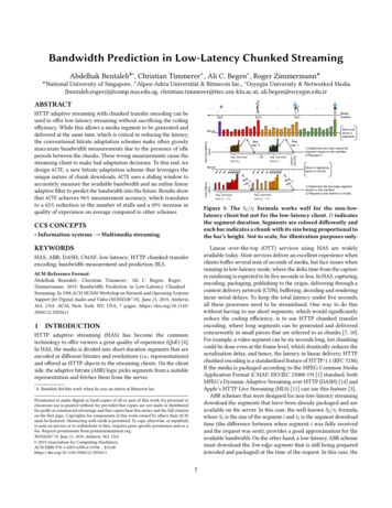
Bandwidth Prediction in Low-Latency Chunked Streaming NationalAbdelhak Bentaleb · , Christian Timmerer , Ali C. Begen , Roger Zimmermann University of Singapore, Alpen-Adria Universität & Bitmovin Inc., Ozyegin University & Networked Media{bentaleb,rogerz}@comp.nus.edu.sg, christian.timmerer@itec.uni-klu.ac.at, ali.begen@ozyegin.edu.trABSTRACTHTTP adaptive streaming with chunked transfer encoding can beused to offer low-latency streaming without sacrificing the codingefficiency. While this allows a media segment to be generated anddelivered at the same time, which is critical in reducing the latency,the conventional bitrate adaptation schemes make often grosslyinaccurate bandwidth measurements due to the presence of idleperiods between the chunks. These wrong measurements cause thestreaming client to make bad adaptation decisions. To this end, wedesign ACTE, a new bitrate adaptation scheme that leverages theunique nature of chunk downloads. ACTE uses a sliding window toaccurately measure the available bandwidth and an online linearadaptive filter to predict the bandwidth into the future. Results showthat ACTE achieves 96% measurement accuracy, which translatesto a 65% reduction in the number of stalls and a 49% increase inquality of experience on average compared to other schemes.3xD0Seg. downloadIdletime (𝜏2)Seg. downloadtime (𝜏1)Sessionstart timeReq.seg. 1Req.seg. neStore andserve insegmentsServer1) Determine the most recent fullsegment based on the manifest2) Request itStore in segments,serve in chunksq.Re . 3gseq.Re . 2gseSeg. downloadSeg. downloadtime (𝜏3* D)time (𝜏2* D)1) Determine the live-edge segmentbased on the manifest2) Request it and receive in chunksFigure 1: The Si /τi formula works well for the non-lowlatency client but not for the low-latency client. D indicatesthe segment duration. Segments are colored differently andeach bar indicates a chunk with its size being proportional tothe bar’s height. Not to scale, for illustration purposes only. Information systems Multimedia streaming.KEYWORDSLinear over-the-top (OTT) services using HAS are widelyavailable today. Most services deliver an excellent experience whenclients buffer several tens of seconds of media, but face issues whenrunning in low-latency mode, where the delta time from the captureto rendering is expected to be five seconds or less. In HAS, capturing,encoding, packaging, publishing to the origin, delivering through acontent delivery network (CDN), buffering, decoding and renderingincur serial delays. To keep the total latency under five seconds,all these processes need to be streamlined. One way to do thiswithout having to use short segments, which would significantlyreduce the coding efficiency, is to use HTTP chunked transferencoding, where long segments can be generated and deliveredconcurrently in small pieces that are referred to as chunks [7, 10].For example, a video segment can be six seconds long, but chunkingcould be done even at the frame level, which drastically reduces theserialization delay, and hence, the latency in linear delivery. HTTPchunked encoding is a standardized feature of HTTP/1.1 (RFC 7230).If the media is packaged according to the MPEG Common MediaApplication Format (CMAF; ISO/IEC 23000-19) [1] standard, bothMPEG’s Dynamic Adaptive Streaming over HTTP (DASH) [14] andApple’s HTTP Live Streaming (HLS) [11] can use this feature [3].ABR schemes that were designed for non-low-latency streamingdownload the segments that have been already packaged and areavailable on the server. In this case, the well-known Si /τi formula,where Si is the size of the segment i and τi is the segment downloadtime (the difference between when segment i was fully receivedand the request was sent), provides a good approximation for theavailable bandwidth. On the other hand, a low-latency ABR schememust download the live-edge segment that is still being prepared(encoded and packaged) at the time of the request. In this case, theHAS; ABR; DASH; CMAF; low-latency; HTTP chunked transferencoding; bandwidth measurement and prediction; RLS.ACM Reference Format:Abdelhak Bentaleb, Christian Timmerer , Ali C. Begen , RogerZimmermann. 2019. Bandwidth Prediction in Low-Latency ChunkedStreaming. In 29th ACM SIGMM Workshop on Network and Operating SystemsSupport for Digital Audio and Video (NOSSDAV’19), June 21, 2019, Amherst,MA, USA. ACM, New York, NY, USA, 7 pages. NHTTP adaptive streaming (HAS) has become the commontechnology to offer viewers a great quality of experience (QoE) [4].In HAS, the media is divided into short-duration segments that areencoded at different bitrates and resolutions (i.e., representations)and offered as HTTP objects to the streaming clients. On the clientside, the adaptive bitrate (ABR) logic picks segments from a suitablerepresentation and fetches them from the server. A.1xDServerCCS CONCEPTS12xDBentaleb did this work when he was an intern at Bitmovin Inc.Permission to make digital or hard copies of all or part of this work for personal orclassroom use is granted without fee provided that copies are not made or distributedfor profit or commercial advantage and that copies bear this notice and the full citationon the first page. Copyrights for components of this work owned by others than ACMmust be honored. Abstracting with credit is permitted. To copy otherwise, or republish,to post on servers or to redistribute to lists, requires prior specific permission and/or afee. Request permissions from permissions@acm.org.NOSSDAV’19, June 21, 2019, Amherst, MA, USA 2019 Association for Computing Machinery.ACM ISBN 978-1-4503-6298-6/19/06. . . 15.00https://doi.org/10.1145/3304112.33256117
NOSSDAV’19, June 21, 2019, Amherst, MA, USAA. Bentaleb et al.assisted the players in their requests, while the latter developedan HTML5 MSE player with CMAF low-latency support. Houzé etal. [9] designed a low-latency solution that benefits from multipathcapabilities and chunked transfer encoding. It splits and downloadsmultiple video frames from different paths taking the frame sizesinto account. Shuai et al. [13] analyzed the impact of the playerbuffer occupancy on live streaming and proposed an ABR schemebased on buffer stabilization for low latency with two-secondsegments. van der Hooft et al. [17] described an HTTP/2 push-basedapproach for low-latency live streaming with super short segmentswithout using CMAF or chunked transfer encoding. Regardingthe implementation of CMAF low latency, DASH-IF and Akamaiprovided a proof-of-concept in the dash.js player [10]. For moredetails about different ABR schemes, refer to [4].The studies mentioned above show good performance in certainnetwork environments and under certain assumptions. However,none of them has systematically analyzed how to effectively selecta good bitrate in the context of various network conditions withthe explicit aim of maintaining a low latency while utilizing CMAF.chunks of the segment that are already available are sent to theclient as fast as possible (transmission is network-limited), whereasthe portions that are yet to be prepared will be sent to the client asthey become available (transmission will be source-limited), leavingidle periods between the chunks, as illustrated in Figure 1. Thepresence of idle periods causes the Si /τi formula to fail [10].In the low-latency mode (bottom of Figure 1), chunks in asegment are delivered with relatively more consistent timing(τi D) since the transmission is source-limited. Note that if thenetwork cannot sustain the selected bitrate, the transmission will benetwork-limited and the ABR logic naturally needs to downshift toa lower bitrate. That is, the download time for a segment cannot beshorter than its duration (except for the first few segments, whichcould be partially available already when the client’s request hasbeen received by the server). Thus, an ABR scheme naively usingthe Si /τi formula will always find a value equal to (or slightlysmaller than) the segment encoding bitrate. This prevents the clientfrom switching to a higher bitrate representation even when thereis enough available bandwidth in the network to support higherbitrate representations (cf. Section 3.1 for more details). Clearly,we need a new chunk-aware bandwidth measurement method thattakes the idle periods between the chunks into account.This paper presents ACTE: ABR for Chunked Transfer Encoding.ACTE performs accurate bandwidth measurement and prediction inlow-latency streaming, and relies on three main components:3 THE ACTE SCHEME3.1 Low-Latency Data CollectionTo understand the effects of ABR and its behavior with low-latencystreaming, we collected data of a real-time video session fromthe Twitch platform with low-latency mode enabled. We usedWireshark and our Web crawler based on the Twitch API-v51 tocollect packet and application-level data, respectively. There weretwo reasons for selecting Twitch: (i) its CMAF low-latency support,and (ii) the Twitch API-v5, which allows to collect various livestreaming session information and metrics like bitrate, resolution,buffer size, total latency, etc., in real time.We used a Scrapy-based2 crawler to collect twelve hours ofTwitch data from a channel at different times during a weekin November 2018. We logged the data in a CSV file every 100milliseconds. During the data collection, we ran traffic shapingon a proxy using tc-NetEm3 to emulate a real last-mile link withvarying network conditions (profile BW3 , see Table 2). The proxywas located on the client side and played the role of an intermediarybetween the client and Twitch server. To measure the bandwidth ( Si /τi ), we used the packet-level data collected with Wireshark, inparticular, the segment sizes as well as segment request and arrivaltimes. The video of the live channel was encoded at six bitratelevels of {0.18,0.73,1.83,2.5,3.1,8.8} Mbps with three resolutions of{540p,720p,1080p} conforming to CMAF.(1) Bandwidth Measurement implements a sliding window basedmoving average method to measure chunk-level bandwidth.(2) Bandwidth Prediction implements an online linear adaptivefilter based on an adaptive recursive least squares (RLS)algorithm [8] to predict the bandwidth into the future basedon the measured samples. RLS works well since bandwidthmeasurements are correlated, stationary and deterministic.(3) ABR Controller implements a throughput-based bitrateselection logic that takes bandwidth prediction values asinput and computes the best bitrate to select.We implemented ACTE in the dash.js reference player [6] and offera demo [2]. We analyzed ACTE’s performance on a broad set of realworld network traces with different video parameters, bandwidthmeasurement algorithms and dash.js ABR schemes.The rest of the paper is organized as follows. Related workis provided in Section 2, followed by the details for the ACTEscheme and its implementation in Section 3. Section 4 presentsthe experimental evaluation and Section 5 concludes the paper.2RELATED WORK5Bitrate (Mbps)Swaminathan et al. [16] proposed a low-latency HTTP chunkedencoding based approach that decoupled the live delay from thesegment duration. The approach analytically evaluated the latencyin three live streaming methods, including a (i) segment-basedmethod where the player requested the segment only if it wasfully available, (ii) server-wait method where the player requesteda segment before it was ready at the server, and (iii) chunkedencoding method where the player received chunks before thefull segment was ready. Bouzakaria et al. [5] and El Essaili etal. [7] investigated the adoption of chunked transfer encodingin live DASH delivery systems to reduce latency. The formerintroduced a new timing parameter in the DASH manifest thatBitrate SelectedMeasured Bandwidthtc Bandwidth (BW3 )43210300600900Time (s)Figure 2: Results for CMAF low latency (Twitch).1 https://dev.twitch.tv/2 https://scrapy.org/3 https://wiki.archlinux.org/index.php/advanced traffic control81,200
Bandwidth Prediction in Low-Latency Chunked StreamingNOSSDAV’19, June 21, 2019, Amherst, MA, USAFigure 2 depicts twelve minutes of the collected data in terms ofthe selected bitrate, measured bandwidth (segment-based), and tcbandwidth. As the figure shows, the Twitch player (version 2.6.3139e00d61) always selected the same bitrate of 1.83 Mbps, while themeasured bandwidth ranged from 2 to 2.5 Mbps. The measuredbandwidth clearly does not track the tc bandwidth accurately,resulting in a constant bitrate selection (i.e., no adaptation).(1)mth segmentnth chunkSize: QmnLoggerSize: Qmn 1Size: Qmn 2Motivated by our observations in Section 3.1, we designed ACTE.Figure 3 shows the components of ACTE in the dash.js referenceplayer [6]. It has four components, (1) bandwidth measurement, (2)bandwidth prediction, (3) ABR controller and (4) logger. The list ofnotations used in ACTE is given in Table 1.mth segment(n 1)th chunkACTE Components and FunctionsResponses(In chunks)z 1i nQm1Õ,i ni nz n 0 em bmwhere Q is the chunk size, and b and e are the beginning and endtimes of the chunk download, respectively, as illustrated in Figure 4.(1) requires us to know the values for Q, b and e. Q is inferred fromthe HTTP header and the HTTP Fetch API provides us the valuefor e. However, with the standard HTTP protocol we have no meansto determine the value for b. If there is a non-negligible idle periodn 1 e n 0), that chunkafter a chunk is downloaded (i.e., when bmmmust be disregarded in computing (1). Since we do not know the bvalues, we have to determine such chunks in a different way.mth segment(n 2)th chunk3.2ci SegmentRequestsemn 2ABR ControllerAveraging of chunk burst timesBufferABRDecisionSliding WindowBandwidth PredictionDisplayC(i)W(i)Filter Tapsĉi -ci Hybrid ĉi 1𝝐iUpdateFigure 3: ACTE overview in dash.js reference player.Modifications required by ACTE are highlighted in gray.Table 1: List of notations.MeaningMW(i)P(i)G(i)C(i)Rσλiciϵiyi ( ĉ i )ĉ i 1rilil t ar дe tBizKnQmnbmnemFilter lengthFilter taps (coefficients) vector of length MThe inverse correlation matrix of size M MThe gain vector of length MMost recent bandwidth measurements of length MList of bitrate levelsInitial input variance estimate parameter for P(0)Forgetting factorChunk downloading stepMeasured average bandwidth at step iEstimated error at step iThe bandwidth prediction at step iBandwidth prediction for the next step (step i 1)Bitrate level selected at step iCurrent latency at step iTarget latencyBuffer level at step iSliding window size for bandwidth measurementsTotal number of downloaded chunksSize of the m t h segment’s n t h chunkBeginning time of the chunk downloadEnd time of the chunk downloademnbmnMediatimelineFirst, we assume that the server pushes the chunks at full networkspeed, and thus, the idle periods could only happen between thechunks of a particular segment, not within a chunk. We downloadevery chunk into a partial buffer such that the sum of all partialbuffers constitutes the respective segment. For each chunk n (forn ) by thesegment m), we divide the size of the partial buffer (Qmn 1 ) and thedelta time between the previous chunk’s end time (emn ). If this download rate is close to thecurrent chunk’s end time (em ), it implies there isaverage download rate of the segment (Sm /τmn 1nnon-negligible idle period from em to em , and this chunk must bedisregarded in computing (1). If not, the idle period is negligible andthe chunk download rate is a good approximation of the availablebandwidth, thus, should be used in (1).Buffer-basedNotationemn 1 bmn 1Figure 4: The idle periods between the chunks of a segment.Throughput-basedBandwidth Measurementbmn 23.2.2 Bandwidth Prediction. This component implements a linearhistory-based prediction, in particular, an online linear adaptivefilter that is based on a recursive least squares (RLS) approach [8].This procedure is presented in Algorithm 1, where for each chunkdownloading step i, it takes as an input a vector of the M mostrecent bandwidth measurement values C(i) given by the bandwidthmeasurement component (BW-Measurement), and then recursivelycomputes the gain vector G(i), the inverse correlation matrixP(i) of the bandwidth measurement values, and the estimatederror ϵi . These values are then used to update the filter tapsvector W(i) of length M, and finally return the future bandwidthprediction for the next step ĉ i 1 ( W(i) C(i)) (see line 12 inAlgorithm1). We used RLS for three main reasons. First, it isfrequently used in practical real-time systems when there is alimitation in computational capabilities. Second, it does not needa prediction model for its input, and third, it leverages the factthat measured bandwidth values are correlated, stationary anddeterministic. Moreover, the proposed algorithm is robust againsttime-varying network conditions through the forgetting factor λ,where this factor does not rely on the time-evolution model forthe system, and in contrast, gives exponentially less weight to thepast bandwidth measurements. For accurate bandwidth prediction,our algorithm strives to minimize the error (min ϵi ) between the3.2.1 Bandwidth Measurement. This component implements thesliding window moving average bandwidth measurement method,which computes the average bandwidth for the last z successfulchunk downloads, where z 3 in ACTE. At each chunk downloadingstep i, the average bandwidth is calculated as follows:9
NOSSDAV’19, June 21, 2019, Amherst, MA, USAA. Bentaleb et al.next (step i 1) bandwidth measurement and the current (step i)future bandwidth prediction. The computational complexity andoverhead of our algorithm is low depending on the filter length M.The overall complexity is O(M 2 ) per time iteration.measurement algorithms: segment-based last bandwidth (SLBW),chunk-based exponentially weighted moving average (EWMA),chunk-based sliding window moving average (SWMA) and Will’ssimple slide-load (WSSL) [10], (v) ABR schemes of throughputbased (TH), buffer-based (BOLA) and hybrid (TH BOLA, referredto as Dynamic), and (vi) QoE metrics of average bitrate, startupdelay, stall duration and number of bitrate switches.Algorithm 1 Bandwidth Prediction (RLS-based)1:2:3:4:5:6:7:8:9:10:11:12:13:W(0) 0, P(0) I σ 1 , ϵ 0, C(0) 0σ 0.001, λ 0.999, BW-Measurement Sliding-Window()function ACTEUpdate()for Each chunk downloading step i 0 do 1 1)C(i 1)G(i) 1 CλT (iP(i 1)P(i 1)C(i 1)P(i) λ 1 P(i 1) λ 1 G(i) CT (i 1) P(i 1)c i Sliding-Window()yi ĉ i WT (i 1) C(i 1)ϵi c i yiC(i) Update(c i )W(i) W(i 1) ϵi G(i)ĉ i 1 W(i) C(i)Return(ĉ i 1 )4.1Methodology4.1.1 Bandwidth Variation Profiles. As shown in Table 2, we usedthree network profiles in the evaluation, denoted BW1 , BW2 andBW3 . These profiles correspond to the DASH-IF guidelines for areal-world bandwidth measurement dataset [6, 15] and follow thecascade pattern (high-low-high and low-high-low). Each profileconsists of different bandwidth values, round-trip times (RTT; inmilliseconds), packet loss rates (in %) and bandwidth variationdurations (in seconds).Table 2: Bandwidth variation profiles.3.2.3 ABR Controller. This component implements three mainheuristic-based ABR schemes that are (1) throughput-based: usingthe measured bandwidth to perform the ABR decisions, (2) bufferbased (BOLA): using the playback buffer occupancy [15] to performthe ABR decisions, and (3) hybrid: a combination of throughputbased and buffer-based. It also monitors the playback bufferoccupancy through the buffer controller component to avoidstalls and maintains the buffer occupancy within a safe region(between minimum and maximum predefined thresholds for CMAFlow latency). ACTE relies on the throughput-based ABR scheme,which is in turn based on the bandwidth measurement andbandwidth prediction components described above. At every chunkdownloading step i, the ACTE ABR scheme takes the bandwidthprediction value ĉ i 1 as input and then outputs the optimal bitratelevel. The objective function F is defined as:F: find r i , arg min ϵi and arg max QoEi s.t. l i l t ar дe t , c i yi , and r i ĉ i 10.5 B i l t ar дe t ,NetworkProfileBW1BW2BW3Inter-variationDuration (s)3030304.1.2 Video Parameters. We used the short movie Tears of Steel 4for the evaluation. Each segment is six seconds long and encodedinto three bitrate levels for video at {0.7, 1.3 and 2.0} Mbps andone bitrate level for audio at 96 Kbps. The chunk duration is 500milliseconds, the target latency is set to 3.2 seconds, and each livestreaming session is 560 seconds long. These video parametersare predefined based on an existing live service used for thisexperimental evaluation. In the future, we plan more extensiveevaluations requiring a larger scale setup.4.1.3 Bandwidth Measurement and Prediction Parameters. We ranan offline MATLAB-based experiment to find suitable parametervalues (z, M, σ , and λ) for the bandwidth measurement andprediction components that respected our objective function Fand minimized the estimated error ϵ. We investigated the followingvalues: z [2 to 5], M [2 to 5], σ [0.001, 0.01, 0.1], and λ [0.999, 0.5, 0.1]. Figure 5 shows the achieved estimated error asa function of time for ACTE (RLS-based) and Linear Mean Square(LMS) [8] with µ (mean) 0.075. Using z 3, M 3, σ 0.001, andλ 0.999, ACTE was quickly able to minimize the estimated errorfor bandwidth prediction, achieve the best result, and significantlyoutperform the LMS-based bandwidth prediction. i 0,(2)where the objective is to find the optimal bitrate level r i R thatminimizes the estimated error and maximizes the QoE respectingthe target latency lt ar дet [2.5, . . . , 3.2] seconds (keeping thecurrent latency li sufficiently small), current network capacity andcurrent playback buffer occupancy Bi . We note that ACTE performsbitrate changes at segment boundaries, not chunk boundaries.3.2.4 Logger. This component periodically records various metricssuch as the selected bitrate, buffer occupancy, measured/predictedbandwidth values, stalls and startup delay.4Bandwidth Values(Mbps)4, 3.5, 3, 2.5, 3, 3.55, 3, 2.5, 2, 2.5, 3, 5, 35, 2.5, 1.5, 1, 1.5, 2.5, 5, 2.54.1.4 Performance Metrics. We tested the efficiency of our solutionusing four main models: (1) live latency [6], (2) Yin QoE [18], (3)ITU-T Rec. P.1203 QoE (Mode 0) [12], and (4) bandwidth predictionaccuracy. The live latency model is given by the dash.js referenceplayer [6] and represents the total time from capturing to rendering.The ITU-T Rec. P.1203 QoE model in Mode 0 takes as input fourmetrics: bitrate, stall duration, frame rate, and resolution. Howto compute the QoE is described in [12]. This model outputsQoE values in the range of 1 to 5 (MOS), and we normalizedEXPERIMENTAL EVALUATIONWe evaluated the performance of ACTE through a set of realworld trace-driven experiments. Each experiment covers variousoperating regimes and settings including (i) video parameters:bitrate level, resolution, chunk and segment duration, and targetlatency, (ii) bandwidth variation profiles (see Table 2), (iii)bandwidth measurement and prediction parameters, (iv) bandwidth4 https://mango.blender.org/download/10
Estimated Error (ϵ)Bandwidth Prediction in Low-Latency Chunked StreamingNOSSDAV’19, June 21, 2019, Amherst, MA, USATable 3: ABR and bandwidth measurement WMASWMAWSSL10-110-210-30140280420560Time (s)Figure 5: Estimated error in ACTE and LMS.i 1q(r i ) δ 1K 1Õi 1q(r i 1 ) q(r i ) δ 2Ts t al l δ 3Tsd .4.2RMSE K 1 Õ yi c i 2, %accuracy (1 RMSE) 100K i 1ciResultsIn this section, we show the average results for the bandwidthvariation profiles. For accuracy, we repeated all experiments tentimes for each ABR scheme with the same configuration, andall presented results are averages over the ten runs. Figure 6illustrates the error bars (standard deviation) of the average selectedbitrate, average measured bandwidth, and average live latencyfor different ABR schemes. Table 4 highlights the overall averageresults for various performance metrics. Two main observationscan be drawn from these experiments. First, ACTE achieves thebest results, outperforming other ABR schemes on each consideredperformance metric. THwss is the runner-up, achieving the secondbest average N-QoE. Second, other ABR schemes suffer from poorperformance because their bandwidth measurement algorithmsmay give incorrect values, leading to sub-optimal ABR decisions,unsatisfactory QoE and high latency.Figure 6 and Table 4 show that ACTE selects the best bitratesresulting in a total average of 1.6 Mbps ranging from 1.4 to 1.7 Mbps(see Figure 6a), a smaller average number of switches (17), alower average number of stalls (3) and a shorter stall durationof 0.76 seconds, a shorter average startup delay of 0.71 seconds,and thus, a higher average N-QoE of 0.95. This is because of theaccurate bandwidth measurement and prediction employed byACTE, where (i) the SWMA over the last three downloaded chunksoutputs an accurate average bandwidth value (average of 2.6 Mbps),which closely approximates the average bandwidth profile values(see Figure 6b), and (ii) ACTEUpdate() (RLS-based) significantlyimproves the ABR selection for low-latency streaming by offeringthe bandwidth prediction for the next average bandwidth with alow average RMSE of 0.033 and a high average accuracy of 96.63%.All of these ACTE results contribute to achieving a low averagelatency of 2.5 seconds (see Figure 6c), which is close to the averagebuffer occupancy (see Table 4).THwss achieves the second best results (e.g., N-QoE) after ACTEthanks to the TCP active probe-based technique that measuresthe bandwidth accurately by downloading a previous segment(using xhr API) available at the edge server, in parallel with thecurrent chunk. However, this scheme incurs overhead (downloadingredundant segments) that may harm the efficiency of THwss . Forexample, the average number of switches, average number of stallsand average stall duration reach 23, 16 and 9 seconds, respectively,and thus, the average N-QoE as well as live latency are negativelyimpacted. THsl achieves the worst results in terms of average NQoE and live latency. This is due to the fact that THsl alwaysplays the video at the lowest bitrate of 0.7 Mbps because the(3)The four terms of (3) are the average bitrate level, number ofbitrate switches, stall duration and startup delay, respectively. K( 560/0.5 1120) is the total number of chunks, q(.) is a qualityfunction that maps bitrate to quality, δ 1 1, and δ 2 and δ 3 are setto the maximum bitrate level in the bitrate list. To simplify thepresentation of the QoE, we used a normalized QoE (N-QoE) withvalues between 0 and 1. To achieve that, we calculated the optimalachievable QoE (QoE ) offline for each bandwidth variation profilewith the full knowledge of the network conditions using dynamicprogramming (N-QoE QoE / QoE ).The bandwidth prediction accuracy model is based on the RootMean Square Error (RMSE) to compute the differences betweenthe measured and predicted bandwidth values (sample standarddeviation).vutHybridDynamicsw-algorithm combinations used in the experiments. For example, THslindicates that throughput-based (TH) ABR is combined with theSLBW algorithm.them (N-QoEitu ) to [0,1]. The Yin QoE model [18] combines fourperformance metrics into one QoE value as follows:KÕABR SchemesThroughput-based Buffer-basedTHslTHewTHswBOLAswTHw s s-(4)4.1.5 Experimental Setup. Our setup consisted of two machines(running Ubuntu 18.04 LTS). One ran our dash.js player (seeFigure 3) in a Google Chrome browser (v63) and one acted as aproxy to simplify bandwidth shaping between the client and server.The origin and edge servers were Cloudflare servers with CMAFpackaging encoding and delivery enabled. Both machines wereconnected through a router and tc-NetEm was used to shape thenetwork capacity according to our bandwidth variation profiles,including their RTTs and packet loss rates sequentially, as: (38 ms,0.09%), (50 ms, 0.08%), (75 ms, 0.06%), (88 ms,0.09%), (100 ms,0.12%).We set the minimum and maximum buffer thresholds to half asecond and the value of target latency, respectively. Furthermore,we used iPerf to generate random TCP-based cross traffic rangingfrom 0.5 to 2 Mbps. We compared ACTE against a set of dash.jsbased ABR schemes with different configurations of bandwidthmeasurement algorithms. Additionally, we implemented the WSSLalgorithm in the dash.js player. WSSL simultaneously downloadsan earlier segment (that is fully available at the edge) and acurrent one while respecting the buffer occupancy and targetlatency. It then measures the bandwidth based on the redundantsegment download. WSSL is an active probe-based technique thatstarts at every segment boundary and backs off immediately ifthe player encounters an increased latency (TCP-like congestioncontrol). Table 3 lists the ABR schemes and bandwidth measurement11
NOSSDAV’19, June 21, 2019, Amherst, MA, USAA. Bentaleb et al.Table 4: Average bitrate level, live latency, QoE with its metrics, RMSE and prediction accuracy.(a) Average selected bitrate.Avg. StartupDelay (s)Avg. N-QoE(N-QoEi t u )Avg.RMSEAvg. PredictionAccuracy (%)0.711.461.061.030.881.660.920.95 (0.92)0.42 (0.50)0.60 (0.60)0.76 (0.65)0.85 (0.78)0.65 (0.68)0.74 (0.72)0.033-96.63 %-20(b) Average measured wssTHewTHsl0ACTE14BOLAsw2THwss36THswAvg. Live Latency (s)4THew3 & 0.762 & 0.8621 & 6627 & 3316 & 958 & 11953 & 68THslAvg. # of Stalls& Duration (s)ACTE1701824232030Avg. Bandwidth (Mbps)2.3 to 3.0 (2.5)5.0 to 5.8 (5.4)4.0 to 5.0 (4.5)3.0 to 4.0 (3.6)3.1 to 3.3 (3.2)3.0 to 4.0 (3.6)3.0 to 5.0 (3.9)Dynamicsw2.1 to 3.0 (
3.1 Low-Latency Data Collection To understand the e ects of ABR and its behavior with low-latency streaming, we collected data of a real-time video session from the Twitch platform with low-latency mode enabled. We used Wireshark and our Web crawler based on the Twitch API-v5 1 to collect packet and application-level data, respectively. There were