Transcription
The Computing Landscape of the 21st CenturyMahadev SatyanarayananWei GaoBrandon LuciaCarnegie Mellon Universitysatya@cs.cmu.eduUniversity of PittsburghWEIGAO@pitt.eduCarnegie Mellon Universityblucia@andrew.cmu.eduABSTRACT2This paper shows how today’s complex computing landscape canbe understood in simple terms through a 4-tier model. Each tier represents a distinct and stable set of design constraints that dominateattention at that tier. There are typically many alternative implementations of hardware and software at each tier, but all of them aresubject to the same set of design constraints. We discuss how thissimple and compact framework has explanatory power and predictive value in reasoning about system design.Today’s computing landscape is best understood by the tiered modelshown in Figure 1. Each tier represents a distinct and stable set ofdesign constraints that dominate attention at that tier. There are typically many alternative implementations of hardware and softwareat each tier, but all of them are subject to the same set of designconstraints. There is no expectation of full interoperability acrosstiers — randomly choosing one component from each tier is unlikely to result in a functional system. Rather, there are many setsof compatible choices across tiers. For example, a single companywill ensure that its products at each tier work well with its ownproducts in other tiers, but not necessarily with products of othercompanies. The tiered model of Figure 1 is thus quite different fromthe well-known “hourglass” model of interoperability. Rather thandefining functional boundaries or APIs, the tiered model segmentsthe end-to-end computing path and highlights design commonalities.In each tier there is considerable churn at timescales of up to a fewyears, driven by technical progress as well as market-driven tacticsand monetization efforts. The relationship between tiers, however,is stable over decade-long timescales. A major shift in computingtypically involves the appearance, disappearance or re-purposing ofa tier in Figure 1. We describe the four tiers of Figure 1 in the restof this section. Section 3 then explains how the tiered model canused as an aid to reasoning about the design of a distributed system.Section 4 examines energy relationships across tiers. Section 5 interprets the past six decades of computing in the context of Figure 1,and Section 6 speculates on the future.ACM Reference Format:Mahadev Satyanarayanan, Wei Gao, and Brandon Lucia. 2019. The Computing Landscape of the 21st Century. In The 20th International Workshopon Mobile Computing Systems and Applications (HotMobile ’19), February27–28, 2019, Santa Cruz, CA, USA. ACM, New York, NY, USA, 6 oductionThe creation of the Periodic Table in the late nineteenth and earlytwentieth centuries was an exquisite intellectual feat [36]. In a smalland simple data structure, it organizes our knowledge about allthe elements in our universe. The position of an element in thetable immediately suggests its physical attributes and its chemicalaffinities to other elements. The presence of “holes” in early versionsof the table led to the search and discovery of previously unknownelements with predicted properties. This simple data structure haswithstood the test of time. As new man-made elements were created,they could all be accommodated within the existing framework. Thequest to understand the basis of order in this table led to majordiscoveries in physics and chemistry. The history of the periodictable teaches us that there is high value in distilling and codifyingtaxonomical knowledge into a compact form.Today, we face a computing landscape of high complexity thatis reminiscent of the scientific landscape of the late 19th century.Is there a way to organize our computing universe into a simpleand compact framework that has explanatory power and predictivevalue? What is our analog of the periodic table? In this paper, wedescribe our initial effort at such an intellectual distillation. Theperiodic table took multiple decades and the contributions of manyresearchers to evolve into the familiar form that we know today.We therefore recognize that this paper is only the beginning of animportant conversation in the research community.2.1A Tiered Model of ComputingTier-1: Elasticity, Permanence and ConsolidationTier-1 represents “the cloud” in today’s parlance. Two dominantthemes of Tier-1 are compute elasticity and storage permanence.Cloud computing has almost unlimited elasticity, as a Tier-1 datacenter can easily spin up servers to rapidly meet peak demand. Relative to Tier-1, all other tiers have very limited elasticity. In terms ofarchival preservation, the cloud is the safest place to store data withconfidence that it can be retrieved far into the future. A combinationof storage redundancy (e.g., RAID), infrastructure stability (i.e., datacenter engineering), and management practices (e.g., data backupand disaster recovery) together ensure the long-term integrity andaccessibility of data entrusted to the cloud. Relative to the data permanence of Tier-1, all other tiers offer more tenuous safety. Gettingimportant data captured at those tiers to the cloud is often an imperative. Tier-1 exploits economies of scale to offer very low total costsof computing. As hardware costs shrink relative to personnel costs,it becomes valuable to amortize IT personnel costs over many machines in a large data center. Consolidation is thus a third dominanttheme of Tier-1. For large tasks without strict timing, data ingressvolume, or data privacy requirements, Tier-1 is typically the optimalplace to perform the task.Permission to make digital or hard copies of part or all of this work for personal orclassroom use is granted without fee provided that copies are not made or distributedfor profit or commercial advantage and that copies bear this notice and the full citationon the first page. Copyrights for third-party components of this work must be honored.For all other uses, contact the owner/author(s).HotMobile ’19, February 27–28, 2019, Santa Cruz, CA, USA 2019 Copyright held by the owner/author(s).ACM ISBN 978-1-4503-6273-3/19/02.https://doi . org/10 . 1145/3301293 . 33023571
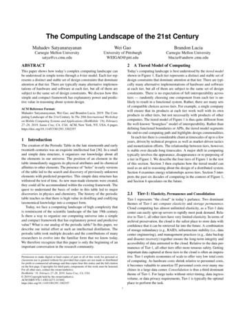
CloudletsRFID TagSwallowableCapsuleImmersive proximityRobotic InsectDronesStatic & VehicularSensor ArraysSmartphonesWiFi BackscatterDeviceTier 4MicrosoftHololens Magic LeaplowlatencyhighbandwidthLuggableWide-Area NetworkVehicularwirelessnetworkAR/VR DevicesMiniMini-datacenterTier 3Tier 2Tier 1Figure 1: Four-tier Model of Computing2.2Tier-3: Mobility and SensingWe consider Tier-3 next, because understanding its attributes helpsto define Tier-2. Mobility is a defining attribute of Tier-3 because itplaces stringent constraints on weight, size, and heat dissipation ofdevices that a user carries or wears [29]. Such a device cannot be toolarge, too heavy or run too hot. Battery life is another crucial designconstraint. Together, these four constraints severely limit designs atTier-3. Technological breakthroughs (e.g., a new battery technologyor a new lightweight and flexible display material) may expand theenvelope of designs, but the underlying constraints always remain.Sensing is another defining attribute of Tier-3. Today’s mobile devices are rich in sensors such as GPS, microphones, accelerometers,gyroscopes, and video cameras. Unfortunately, a mobile device maynot be powerful enough to perform real-time analysis of data captured by its on-board sensors (e.g., video analytics). While mobilehardware continues to improve, there is always a large gap betweenwhat is feasible on a mobile device and what is feasible on a serverof the same technological era. Figure 2 shows this large performancegap persisting over a 20-year period from 1997 to 2017. One canview this stubborn gap as a “mobility penalty” — i.e., the price onepays in performance foregone in order to meet mobility constraints.To overcome this penalty, a mobile device can offload computation over a wireless network to Tier-1. This was first described byNoble et al [25] in 1997, and has since been extensively exploredby many others [8, 32]. For example, speech recognition and natural language processing in iOS and Android nowadays work byoffloading their compute-intensive aspects to the cloud.IoT devices can be viewed as Tier-3 devices. Although they maynot be mobile, there is a strong incentive for them to be inexpensive.Since this typically implies meager processing capability, offloadingcomputation to Tier-1 is again attractive.2.3YearTypical Tier-1 ServerProcessorSpeedTypical Tier-3 DeviceDeviceSpeed199720022007Pentium IIItaniumIntel Core 2Palm PilotBlackberry 5810Apple iPhone16 MHz133 MHz412 MHz2011Intel XeonX5Intel XeonE5-2697v2Samsung Galaxy S22.4 GHz(2 cores)6.4 GHz(4 cores)2.4 GHz(2 cores)7.5 GHz(4 cores)4.16 GHz(4 cores)9.4 GHz(4 cores)2013266 MHz1 GHz9.6 GHz(4 cores)32 GHz(2x6 cores)64 GHz(2x12 cores)Samsung Galaxy S4Google Glass2016Intel XeonE5-2698v488.0 GHz(2x20 cores)Samsung Galaxy S7HoloLens2017Intel XeonGold 614896.0 GHz(2x20 cores)Pixel 2Source: Adapted from Chen [3] and Flinn [8]“Speed” metric number of cores times per-core clock speed.Figure 2: The Mobility Penalty: Impact of Tier-3 ConstraintsTier-2 addresses these negative consequences by creating the illusion of bringing Tier-1 “closer.” This achieves two things. First,it enables Tier-3 devices to offload compute-intensive operationsat very low latency. This helps to preserve the tight response timebounds needed for immersive user experience (e.g., augmented reality (AR)) and cyber-physical systems (e.g., drone control). Proximityalso results in a much smaller fan-in between Tiers-3 and -2 thanis the case when Tier-3 devices connect directly to Tier-1. Consequently, Tier-2 processing of data captured at Tier-3 avoids excessivebandwidth demand anywhere in the system. Server hardware at Tier2 is essentially the same as at Tier-1 (i.e., the second column ofFigure 2), but engineered differently. Instead of extreme consolidation, servers in Tier-2 are organized into small, dispersed datacenters called cloudlets. A cloudlet can be viewed as “a data centerin a box.” When a Tier-3 component such as a drone moves far fromits current cloudlet, a mechanism analogous to cellular handoff isrequired to discover and associate with a new optimal cloudlet [9].The introduction of Tier-2 is the essence of edge computing [33].Note that “proximity” here refers to network proximity rather thanphysical proximity. It is crucial that RTT be low and end-to-endbandwidth be high. This is achievable by using a fiber link betweena wireless access point and a cloudlet that is many tens or evenhundreds of kilometers away. Conversely, physical proximity doesnot guarantee network proximity. A highly congested WiFi networkmay have poor RTT, even if Tier-2 is physically near Tier-3.Tier-2: Network ProximityAs mentioned in Section 2.1, economies of scale are achieved in Tier1 by consolidation into a few very large data centers. Extreme consolidation has two negative consequences. First, it tends to lengthennetwork round-trip times (RTT) to Tier-1 from Tier-3 — if there arevery few Tier-1 data centers, the closest one is likely to be far away.Second, the high fan-in from Tier-3 devices implies high cumulativeingress bandwidth demand into Tier-1 data centers. These negative consequences stifle the emergence of new classes of real-time,sensor-rich, compute-intensive applications [34].2
Tier-4: Longevity and OpportunismImportance of Energyin Design (not to scale)2.4A key driver of Tier-3 is the vision of embedded sensing, in whichtiny sensing-computing-communication platforms continuously report on their environment. “Smart dust” is the extreme limit of thisvision. The challenge of cheaply maintaining Tier-3 devices in thefield has proved elusive because replacing their batteries or chargingthem is time-consuming and/or difficult.This has led to the emergence of devices that contain no chemicalenergy source (battery). Instead, they harvest incident EM energy(e.g., visible light or RF) to charge a capacitor, which then powers abrief episode of sensing, computation and wireless transmission. Thedevice then remains passive until the next occasion when sufficientenergy can be harvested to power another such episode. This modality of operation, referred to as intermittent computing [17, 18, 21],eliminates the need for energy-related maintenance of devices inthe field. This class of devices constitutes Tier-4 in the taxonomy ofFigure 1. Longevity of deployment combined with opportunism inenergy harvesting are the distinctive attributes of this tier.The most successful Tier-4 devices today are RFID tags, whichare projected to be a roughly 25 billion market by 2020 [27]. Moresophisticated devices are being explored in research projects including, for example, a robotic flying insect powered solely by anincident laser beam [12]. A Tier-3 device (e.g., RFID reader) provides the energy that is harvested by a Tier-4 device. Immersiveproximity is thus the defining relationship between Tier-4 and Tier-3devices — they have to be physically close enough for the Tier-4device to harvest sufficient energy for an episode of intermittentcomputation. Network proximity alone is not sufficient. RFID readers have a typical range of a few meters today. A Tier-4 device stopsfunctioning when its energy source is misaimed or too far away.3TIER 4TIER 3TIER 14 orders of magnitude10-810-6RFID TagsTIER 210-3 10-2 10-1 100 101 102 103 104 105 106MicrocontrollersEnergy p PCsPowerBudget (W)Data centersTower serversFigure 3: Importance of Energy as a Design Constrainttier severely constrain its range of acceptable designs. A mobiledevice, for example, has to be small, lightweight, energy-efficientand have a small thermal footprint. This imperative follows directlyfrom the salient attribute of mobility. A product that does not meetthis imperative will simply fail in the marketplace.The same reasoning also applies to software at each tier. Forexample, Tier-3 to Tier-1 communication is (by definition) over aWAN and may involve a wireless first hop that is unreliable and/orcongested. Successful Tier-3 software design for this context has toembody support for disconnected and weakly-connected operation.On the other hand, Tier-3 to Tier-2 communication is expected tobe LAN or WLAN quality at all times. A system composed of justthose tiers can afford to ignore support for network failure. Notethat the server hardware in the two cases may be identical: locatedin a data center (Tier-1) or in a closet nearby (Tier-2). It is only theplacement and communication assumptions that are different.Constraints serve as valuable discipline in system design. Although implementation details of competing systems with comparable functionality may vary widely, their tier structure offers a common viewpoint from which to understand their differences. Somedesign choices are forced by the tier, while other design choices aremade for business reasons, for compatibility reasons with productsin other tiers, for efficiency, usability, aesthetics, and so on. Comparison of designs from a tier viewpoint helps to clarify and highlightthe essential similarities versus incidental differences.Like the periodic table mentioned in Section 1, Figure 1 distillsa vast space of possibilities (i.e., design choices for distributed systems) into a compact intellectual framework. However, the analogyshould not be over-drawn since the basis of order in the two worlds isvery different. The periodic table exposes order in a “closed-source”system (i.e., nature). The tiered model reveals structure in an “opensource” world (i.e., man-made system components). The key insightof the tiered model is that, in spite of all the degrees of freedomavailable to designers, the actual designs that thrive in the real worldhave deep structural similarities.Using the ModelThe tiers of Figure 1 can be viewed as a canonical representation ofcomponents in a modern distributed system. Of course, not everydistributed system will have all four tiers. For example, a team ofusers playing Pokemon Go will only use smartphones (Tier-3) anda server in the cloud (Tier-1). A worker in a warehouse who istaking inventory will use an RFID reader (Tier-3) and passive RFIDtags that are embedded in the objects being inventoried (Tier-4).A more sophisticated design of this inventory control system mayallow multiple users to work concurrently, and to use a cloudlet inthe warehouse (Tier-2) or the cloud (Tier-1) to do aggregation andduplicate elimination of objects discovered by different workers. Ingeneral, one can deconstruct any complex distributed system andthen examine the system from a tier viewpoint. Such an analysis canbe a valuable aid to deeper understanding of the system.As discussed in Section 2, each tier embodies a small set of salientproperties that define the reason for the existence of that tier. Elasticity, permanence and consolidation are the salient attributes ofTier-1; mobility and sensing are those of Tier-3; network proximityto Tier-3 is the central purpose of Tier-2; and, longevity combinedwith opportunism represents the essence of Tier-4. These salientattributes shape both hardware and software designs that are relevantto each tier. For example, hardware at Tier-3 is expected to be mobile and sensor-rich. Specific instances (e.g., a static array of videocameras) may not embody some of these attributes (i.e., mobility),but the broader point is invariably true. The salient attributes of a4The Central Role of EnergyA hidden message of Section 2 is that energy plays a central rolein segmentation across tiers. As shown in Figure 3, the power concerns at different tiers span many orders of magnitude, from a fewnanowatts (e.g., a passive RFID tag) to tens of megawatts (e.g., anexascale data center). Energy is also the most critical factor whenmaking design choices in other aspects of a computing system. For3
example, the limited availability of energy could severely limit performance. The power budget of a system design could also be amajor barrier to reductions of system cost and form factor. The relative heights of tiers in Figure 3 are meant to loosely convey theextent of energy’s influence on design at that tier.Tier-1 (Data Centers): Power is used in a data center for IT equipment (e.g., servers, networks, storage, etc) and infrastructure (e.g.,cooling systems), adding up to as much as 30 MW at peak hours [6].Current power saving techniques focus on load balancing and dynamically eliminating power peaks. Power oversubscription enablesmore servers to be hosted than theoretically possible, leveraging thefact that their peak demands rarely occur simultaneously.Tier-2 (Cloudlets): Cloudlets can span a wide range of form factors,from high-end laptops and desktop PCs to tower or rack servers.Power consumption can therefore can vary from 100W to severalkilowatts. At this tier, well-known power saving techniques suchas CPU frequency scaling [14] are applicable. Techniques havealso been developed to reduce the power consumption of attachedhardware (e.g., GPUs) [23], and to balance the power consumptionamong multiple interconnected cloudlets. As Figure 3 suggests,energy constraints are relatively easy to meet at this tier.Tier-3 (Smartphones): Smartphones are the dominant type of computing device at Tier-3. Their power consumption is below 1000 mWwhen idle [22], but can peak at 3500-4000 mW. Techniques suchas frequency scaling, display optimization, and application partitioning are used to reduce power consumption. Workload-specifictechniques are also used in web browsing and mobile gaming.Tier-3 (Wearables): Studies have shown that the energy consumption of smartwatches can be usually controlled to below 100 mWin stand-by mode with screen off [16]. When the screen is on orthe device is wirelessly transmitting data, the energy consumptioncould surge to 150-200 mW. Various techniques have been proposedto further reduce smartwatch power consumption to 100 mW inactive modes via energy-efficient storage or display management.Tier-4: Energy-harvesting enables infrastructure-free, low-maintenance operation for tiny devices that sense, compute and communicate.Energy harvesting presents unique challenges: sporadic power islimited to 10 7 to 10 8 watts using, e.g., RF or biological sources. Apassive RFID tag consumes hundreds of nA at 1.5V [26]. Emergingwireless backscatter networking enables communication at extremelylow power [15]. Intermittent computing allows sensing and complex processing on scarce energy [5, 17]. Such capabilities enablea new breed of sensors and actuators deployed in the human bodyto monitor health signals, in civil infrastructure, and in adversarialenvironments like outer space [5]. RF beamforming extends thecapability of batteryless, networked, in-vivo devices [19].5The figure at the top is from the 1986 description of the Andrew project by Morris etal [24]. The cloud-like Tier-1 entity (“VICE file system”) offers storage permanencefor the Tier-2 entities at the periphery (“VIRTUE workstations”). The verbatim comments about mobility and system administration are from a 1990 paper [28] aboutthis model of computing.Figure 4: Limited Re-Creation of Tier-1 in a Tier-2 WorldThe emergence of timesharing by the late 1960s introduced elasticity to Tier-1. In a batch-processing system, a job was queued,and eventually received exclusive use of the mainframe. Queueingdelays increased as more jobs competed for the mainframe, therebyexposing the inelasticity of this computing resource. Timesharingmultiplexed the mainframe at fine granularity, rather than seriallyreusing it. It leveraged human think times to provide the illusion thateach user had exclusive access to Tier-1. This illusion broke downat very high load by the increase in queueing delays for user interactions. Until that breaking point, however, Tier-1 appeared elastic tovarying numbers of users. The introduction of virtual machine (VM)technology by the late 1960s expanded this illusion beyond userlevel code. Now, elasticity applied to the entire vertical stack fromlow-level device drivers, through the (guest) operating system, to thetop of the application stack. Many decades later, this encapsulatingability led to the resurgence of VMs in cloud computing.Frustration with the queueing delays of timesharing led to theemergence of personal computing. In this major shift, Tier-1 wascompletely replaced by the brand-new Tier-2. An enterprise thatswitched from timesharing to personal computing was effectivelydisaggregating its consolidated Tier-1 infrastructure into a largenumber of dispersed Tier-2 devices. The dedication of a Tier-2device to each user, combined with its physical proximity to the user,led to crisp interactive response. This, in turn, led to the emergenceof a new class of latency-sensitive applications such as spreadsheets.A spreadsheet does not seem latency-sensitive today, but in the early1980s its latency constraints could only be met at Tier-2.An unintended consequence of the disaggregation of Tier-1 intodispersed Tier-2 elements was its negative impact on shared data.By the early 1980s, the archival data stored in its computing systemwas often of high value to an enterprise. Over the previous decade,business practices had been transformed by the easy sharing of dataacross timesharing users in an enterprise. The disaggregation ofTier-1 into dispersed Tier-2 devices destroyed the mechanisms fordata sharing across users (e.g., a shared file system). It was at thisA Tiered View of the PastIn the beginning, there was only Tier-1. The batch-processing mainframes of the late 1950s and 1960s represented consolidation in itsextreme form. In this primitive world, there were no representativesof Tier-2, Tier-3 or Tier-4. Those tiers could not emerge until thehardware cost of computing and its physical size had dropped bymany orders of magnitude. The wide-area network shown in Figure 1did not exist, but it was foreshadowed by remote punch card readersand line printers connected via point-to-point links to a mainframe.4
juncture that the third important attribute of Tier-1, namely storagepermanence, came to be recognized as crucial. How to preserve Tier1’s ability to share information easily, securely, and with appropriateaccess controls in a dispersed and fragmented Tier-2 world became amajor challenge. The Andrew project [24] addressed this challengeby re-creating Tier-1 for the limited purpose of storage permanence,as shown in Figure 4. A distributed file system (AFS [10, 35]) createdthe illusion that all of Tier-1 storage was accessible via on-demandcaching at Tier-2 devices. The resulting system provided users withthe ease of data sharing characteristic of Tier-1, while preserving thecrisp interactive response of Tier-2. Today, systems such as DropBoxand Box are modern realizations of this concept.As discussed in Section 2.1, a key attribute of a modern Tier-1data center is its large pool of compute nodes that provide elasticity.This capability was first pioneered by the Cambridge ProcessorBank [1] in the 1979-1988 time period, and by Amoeba, a systemfrom roughly the same timeframe [40].The emergence of Tier-3 coincided with the release of the earliestcomputers (circa 1983) that were small enough to be consideredportable devices. The Radio Shack TRS-80 Model 100 (weighingroughly 1.5 kg and powered by 4 AA batteries) and the CompaqPortable (weighing 13 kg) were two early examples. There wasexplosive innovation in laptop hardware by the late 1980s. Oncethe Internet became widely used (mid-1990s), a key distinctionbetween Tier-2 and Tier-3 was the stability and quality of Internetconnectivity. In contrast to Tier-2 devices, Tier-3 devices typicallyhad wireless connectivity with periods of disconnection and poorconnectivity. The desire to preserve shared enterprise data accesseven when mobile led to the creation of Coda File System [31],which extended Figure 4 to Tier-3 devices.By the mid-1990s handheld mobile devices referred to as personal digital assistants (PDAs) emerged. In the same timeframe,computing hardware had become small and light enough for wearable computers to be created [38]. These extreme optimizations ofTier-3 devices led to the mobility penalty discussed earlier (Section 2.2 and Figure 2). The need to process sensor streams in realtime from these devices led to offloading (originally called “cyberforaging” [30]) from Tier-3 to Tier-1 or Tier-2.6can be mitigated by using the extreme parallelism for redundancy.Future computing systems will extend biology with the mechanicalcapabilities of micro- and nano-robotics. This extension can leadto an inversion of the relative costs of computing and actuation [7].At macro-scale, the energy cost of actuation dominates that of computing; but at nano-scale, computing may dominate. Optimizingcomputing in such systems may lead to a new Tier-5.Blurring boundaries between tiers: Tier boundaries in Figure 1are likely to blur, leading to a continuum of devices with differentpower budgets, computing workloads and manufacturing costs. Themajor drivers of such blurring are advances in the manufacturingtechnologies. Such improvement not only allows a device to undertake more computing workloads with a lower power budget and asmaller form factor, but also fosters new computing models that fullyintegrate heterogeneous computing devices into a universal ecosystem. For example, significant chip-level convergence has occuredacross desktop PCs, laptops and smartphones in the past few years,leading to simpler task migration across these devices.A consequence of such blurring boundaries is that the gap incapabilities between cloudlets at Tier 2 and battery-powered mobiledevices at Tier 3 will diminish. In addition, today’s requirement ofchemical batteries at Tier-3 is likely to be gradually relaxed due tomore advanced energy harvesting and wireless charging technologies. This allows significant reduction of device size and alleviatessome design constraints of mobility. Energy harvesting will alsobe able to provide a much higher power budget, which then allowsa richer set of computing tasks being executed at Tier-4 devices.Consequently, the transition between Tier 3 and Tier 4 will be muchsmoother. This smooth transition will lead to more convenient deployment of embedded computing objects and enable many newcomputing paradigms, such as distributed AI in the future IoT.Quantum Computing: In terms of physical size, energy demandand dependence on external cooling, quantum computers wouldseem to map naturally to Tier-1. However, their widespread adoption requires extensive rework of the entire computing landscape.This includes new programming languages to express probabilisticproblems, new programmable quantum architectures, new compilersthat target emerging quantum machines, and new debugging andverification tools that validate results [4]. We do not yet know howto incorporate such a disruptive change into the tiered model ofFigure 1. For now, quantum computing is an outlier.Future EvolutionOur future computing landscape will include computing modalitiesthat are not covered by Figure 1. We speculate on these modalitiesand their implications in this section.Biological Computer Systems: Future computer systems will beinspired by, rendered in, and extensive of biology. Neuromorphiccomputing is seeing a resurgance with analog [11, 37] and delaybased [20, 39] architectures for neural machine learning. Whileanalogies to biological behavior abound, spanning from circuits, toarchitectures, to software and algorithms, computer system behavioris rarely biological in its efficiency and capability. Other emergingsystems le
Tier-1 represents "the cloud" in today's parlance. Two dominant themes of Tier-1 are compute elasticity and storage permanence. Cloud computing has almost unlimited elasticity, as a Tier-1 data center can easily spin up servers to rapidly meet peak demand. Rela-tive to Tier-1, all other tiers have very limited elasticity. In terms of