Transcription
Depth Estimation via Affinity Learned withConvolutional Spatial Propagation NetworkXinjing Cheng , Peng Wang and Ruigang YangBaidu Research, Baidu mAbstract. Depth estimation from a single image is a fundamental problem incomputer vision. In this paper, we propose a simple yet effective convolutionalspatial propagation network (CSPN) to learn the affinity matrix for depth prediction. Specifically, we adopt an efficient linear propagation model, where the propagation is performed with a manner of recurrent convolutional operation, and theaffinity among neighboring pixels is learned through a deep convolutional neural network (CNN). We apply the designed CSPN to two depth estimation tasksgiven a single image: (1) Refine the depth output from existing state-of-the-art(SOTA) methods; (2) Convert sparse depth samples to a dense depth map by embedding the depth samples within the propagation procedure. The second task isinspired by the availability of LiDAR that provides sparse but accurate depth measurements. We experimented the proposed CSPN over the popular NYU v2 [1]and KITTI [2] datasets, where we show that our proposed approach improves notonly quality (e.g., 30% more reduction in depth error), but also speed (e.g., 2 to5 faster) of depth maps than previous SOTA methods. The codes of CSPN areavailable at: https://github.com/XinJCheng/CSPN.Keywords: Depth estimation, Convolutional spatial propagation1IntroductionDepth estimation from a single image, i.e., predicting per-pixel distance to the camera,has many applications from augmented realities (AR), autonomous driving, to robotics.Given a single image, recent efforts to estimate per-pixel depths have yielded highquality outputs by taking advantage of deep fully convolutional neural networks [3,4]and large amount of training data from indoor [1,5,6] and outdoor [2,7,8]. The improvement lies mostly in more accurate estimation of global scene layout and scales withadvanced networks, such as VGG [9] and ResNet [10], and better local structure recovery through deconvolution operation [11], skip-connections [12] or up-projection [4].Nevertheless, upon closer inspection of the output from a contemporary approach [13](Fig. 1(b)), the predicted depths is still blurry and do not align well with the given imagestructure such as object silhouette.Most recently, Liu et al. [14] propose to directly learn the image-dependent affinitythrough a deep CNN with spatial propagation networks (SPN), yielding better results equal contribution
2X. Cheng, P. Wang and R. 046(h)(e)0.035(i)(j)Fig. 1: (a) Input image; (b) Depth from [13]; (c) Depth after bilateral filtering; (d) Refined depth by SPN [14]; (e) Refined depth by CSPN; (f) Sparse depth samples (500);(g) Ground Truth; (h) Depth from our network; (i) Refined depth by SPN with depthsample; (j) Refined depth by CSPN with depth sample. The corresponding root meansquare error (RMSE) is put at the left-top of each predicted depth map.comparing to the manually designed affinity on image segmentation. However, its propagation is performed in a scan-line or scan-column fashion, which is serial in nature.For instance, when propagating left-to-right, pixels at right-most column must wait theinformation from the left-most column to update its value. Intuitively, depth refinementcommonly just needs a local context rather a global one.Here we propose convolutional spatial propagation networks (CSPN), where thedepths at all pixels are updated simultaneously within a local convolutional context.The long range context is obtained through a recurrent operation. Fig. 1 shows an example, the depth estimated from CSPN (e) is more accurate than that from SPN (d) andBilateral filtering (c). In our experiments, our parallel update scheme leads to significantperformance improvement in both speed and quality over the serial ones such as SPN.Practically, we show that the proposed strategy can also be easily extended to convert sparse depth samples to a dense depth map given corresponding image [15,13]. Thistask can be widely applied in robotics and autonomous cars, where depth perception isoften acquired through LiDAR, which usually generates sparse but accurate depth measurement. By combining the sparse measurements with images, we could generate afull-frame dense depth map. For this task, we consider three important requirementsfor an algorithm: (1) The dense depth map recovered should align with image structures; (2) The depth value from the sparse samples should be preserved, since they areusually from a reliable sensor; (3) The transition between sparse depth samples andtheir neighboring depths should be smooth and unnoticeable. In order to satisfy thoserequirements, we first add mirror connections based on the network from [13], whichgenerates better depths as shown in Fig. 1(h). Then, we tried to embed the propagationinto SPN in order to keep the depth value at sparse points. As shown in Fig. 1(i), it generates better details and lower error than SPN without depth samples (Fig. 1(d)). Finally,changing SPN to our CSPN yields the best result (Fig. 1(j)). As can be seen, our recovered depth map with just 500 depth samples produces much more accurately estimatedscene layouts and scales. We experiment our approach over two popular benchmarksfor depth estimation, i.e.NYU v2 [1] and KITTI [2], with standard evaluation crite-
CSPN3ria. In both datasets, our approach is significantly better (relative 30% improvementin most key measurements) than previous deep learning based state-of-the-art (SOTA)algorithms [15,13]. More importantly, it is very efficient yielding 2-5 accelerationcomparing with SPN. In summary, this paper has the following contributions:1. We propose convolutional spatial propagation networks (CSPN) which is more efficient and accurate for depth estimation than the previous SOTA propagation strategy [14], without sacrificing the theoretical guarantee.2. We extend CSPN to the task of converting sparse depth samples to dense depth mapby using the provided sparse depths into the propagation process. It guarantees thatthe sparse input depth values are preserved in the final depth map. It runs in realtime, which is well suited for robotics and autonomous driving applications, wheresparse depth measurement from LiDAR can be fused with image data.2Related WorkDepth estimating and enhancement/refinement have long been center problems for computer vision and robotics. Here we summarize those works in several aspects withoutenumerating them all due to space limitation.Single view depth estimation via CNN and CRF. Deep neural networks (DCN) developed in recent years provide strong feature representation for per-pixel depth estimationfrom a single image. Numerous algorithms are developed through supervised methods [16,3,4,17], semi-supervised methods [18] or unsupervised methods [19,20,21,22].and add in skip and mirror connections. Others tried to improve the estimated details further by appending a conditional random field (CRF) [23,24,25] and joint training [26,27]. However, the affinity for measuring the coherence of neighboring pixels ismanually designed.Depth Enhancement. Traditionally, depth output can be also efficiently enhanced withexplicitly designed affinity through image filtering [28,29], or data-driven ones throughtotal variation (TV) [30,31] and learning to diffuse [32] by incorporating more priorsinto diffusion partial differential equations (PDEs). However, due to the lack of an effective learning strategy, they are limited for large-scale complex visual enhancement.Recently, deep learning based enhancement yields impressive results on super resolution of both images [33,34] and depths [35,36,37,38]. The network takes low resolution inputs and output the high-resolution results, and is trained end-to-end where themapping between input and output is implicitly learned. However, these methods areonly trained and experimented with perfect correspondent ground-truth low-resolutionand high-resolution depth maps and often a black-box model. In our scenario, both theinput and ground truth depth are non-perfect, e.g.depths from a low cost LiDAR or anetwork, thus an explicit diffusion process to guide the enhancement such as SPN isnecessary.Learning affinity for spatial diffusion. Learning affinity matrix with deep CNN fordiffusion or spatial propagation receives high interests in recent years due to its theoretical supports and guarantees [39]. Maire et al. [40] trained a deep CNN to directly predict the entities of an affinity matrix, which demonstrated good performance on imagesegmentation. However, the affinity is followed by an independent non-differentiable
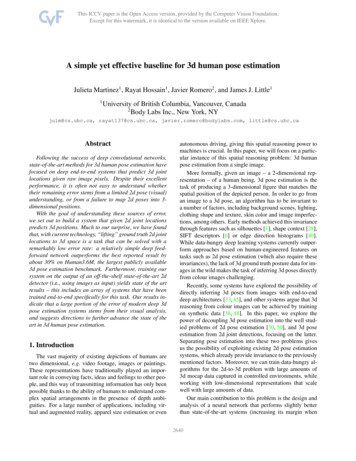
4X. Cheng, P. Wang and R. Yang(a)SPN(b)CSPNFig. 2: Comparison between the propagation process in SPN [14] and CPSN in thiswork.solver of spectral embedding, it can not be supervised end-to-end for the predictiontask. Bertasius et al. [41] introduced a random walk network that optimizes the objectives of pixel-wise affinity for semantic segmentation. Nevertheless, their affinity matrixneeds additional supervision from ground-truth sparse pixel pairs, which limits the potential connections between pixels. Chen et al. [42] try to explicit model an edge mapfor domain transform to improve the output of neural network.The most related work with our approach is SPN [14], where the learning of a largeaffinity matrix for diffusion is converted to learning a local linear spatial propagation,yielding a simple while effective approach for output enhancement. However, as mentioned in Sec. 1, depth enhancement commonly needs local context, it might not benecessary to update a pixel by scanning the whole image. As shown in our experiments,our proposed CSPN is more efficient and provides much better results.Depth estimation with given sparse samples. The task of sparse depth to dense depthestimation was introduced in robotics due to its wide application for enhancing 3Dperception [15]. Different from depth enhancement, the provided depths are usuallyfrom low-cost LiDAR or one line laser sensors, yielding a map with valid depth in onlyfew hundreds of pixels, as illustrated in Fig. 1(f). Most recently, Ma et al. [13] proposeto treat sparse depth map as additional input to a ResNet [4] based depth predictor,producing superior results than the depth output from CNN with solely image input.However, the output results are still blurry, and does not satisfy our requirements ofdepth as discussed in Sec. 1. In our case, we directly embed the sampled depth in thediffusion process, where all the requirements are held and guaranteed.Some other works directly convert sparse 3D points to dense ones without imageinput [43,44,45], whereas the density of sparse points must be high enough to reveal thescene structure, which is not available in our scenario.3Our ApproachWe formulate the problem as an anisotropic diffusion process and the diffusion tensor islearned through a deep CNN directly from the given image, which guides the refinementof the output.
CSPN3.15Convolutional Spatial Propagation NetworkGiven a depth map Do Rm n that is output from a network, and image X Rm n ,our task is to update the depth map to a new depth map Dn within N iteration steps,which first reveals more details of the image, and second improves the per-pixel depthestimation results.Fig. 2(b) illustrates our updating operation. Formally, without loss of generality, wecan embed the Do to some hidden space H Rm n c . The convolutional transformation functional with a kernel size of k for each time step t could be written as,Hi,j,t 1 X(k 1)/2a,b (k 1)/2κi,j (a, b) Hi a,j b,tκ̂i,j (a, b),a,b,a,b6 0 κ̂i,j (a, b) Xκi,j (0, 0) 1 κi,j (a, b)where, κi,j (a, b) Pa,b,a,b6 0(1)where the transformation kernel κ̂i,j Rk k c is the output from an affinity network,which is spatially dependent on the input image. The kernel size k is usually set as anodd number so that the computational context surrounding pixel (i, j) is symmetric. is element-wise product. Following [14], we normalize kernel weights between rangeof ( 1,P 1) so that the model can be stabilized and converged by satisfying the condition a,b,a,b6 0 κi,j (a, b) 1. Finally, we perform this iteration N steps to reach astationary distribution.Correspondence to diffusion process with a partial differential equation (PDE).Similar with [14], here we show that our CSPN holds all the desired properties of SPN.Formally, we can rewrite the propagation in Eq. (1) as a process of diffusion evolutionby first doing column-first vectorization of feature map H to Hv Rmn c . 1 λ0,0 κ0,0 (1, 0) · · ·0 κ1,0 ( 1, 0) 1 λ1,0 · · ·0 GHtv .(2)Ht 1 .v .···· · · 1 λm,nPwhere λi,j a,b κi,j (a, b) and G is a mn mn transformation matrix. The diffusionprocess expressed with a partial differential equation (PDE) is derived as follows,Ht 1 GHtv (I D A)HtvvHt 1 Htv (D A)Htvv t Hvt 1 LHtv(3)where L is the Laplacian matrix, D is the diagonal matrix containing all the λi,j , andA is the affinity matrix which is the off diagonal part of G.In our formulation, different from [14] which scans the whole image in four directions (Fig. 2(a)) sequentially, CSPN propagates a local area towards all directions at
6X. Cheng, P. Wang and R. YangFig. 3: (a) Histogram of RMSE with depth maps from [13] at given sparse depth points.(b) Comparison of gradient error between depth maps with sparse depth replacement(blue bars) and with ours CSPN (green bars), where ours is much smaller. Check Fig. 4for an example. Vertical axis shows the count of pixels.each step (Fig. 2(b)) simultaneously, i.e.with k k local context, while larger context isobserved when recurrent processing is performed, and the context acquiring rate is inan order of O(kN ).In practical, we choose to use convolutional operation due to that it can be efficiently implemented through image vectorization, yielding real-time performance indepth refinement tasks.Principally, CSPN could also be derived from loopy belief propagation with sumproduct algorithm [46]. However, since our approach adopts linear propagation, whichis efficient while just a special case of pairwise potential with L2 reconstruction loss ingraphical models. Therefore, to make it more accurate, we call our strategy convolutional spatial propagation in the field of diffusion process.3.2Spatial Propagation with Sparse Depth SamplesIn this application, we have an additional sparse depth map Ds (Fig. 4(b)) to help estimate a depth depth map from a RGB image. Specifically, a sparse set of pixels areset with real depth values from some depth sensors, which can be used to guide ourpropagation process.Similarly, we also embed the sparse depth map Ds {dsi,j } to a hidden representation Hs , and we can write the updating equation of H by simply adding a replacementstep after performing Eq. (1),Hi,j,t 1 (1 mi,j )Hi,j,t 1 mi,j Hsi,j(4)where mi,j I(dsi,j 0) is an indicator for the availability of sparse depth at (i, j).In this way, we guarantee that our refined depths have the exact same value at thosevalid pixels in sparse depth map. Additionally, we propagate the information from thosesparse depth to its surrounding pixels such that the smoothness between the sparsedepths and their neighbors are maintained. Thirdly, thanks to the diffusion process, thefinal depth map is well aligned with image structures. This fully satisfies the desiredthree properties for this task which is discussed in our introduction (1).
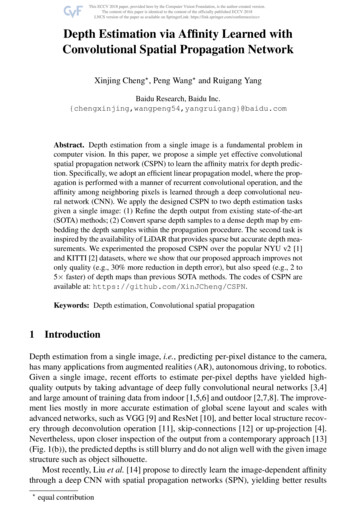
CSPN7(c)(a)(d)(b)DepthSobel xFig. 4: Comparison of depth map [13] with sparse depth replacement and with ourCSPN w.r.t. smoothness of depth gradient at sparse depth points. (a) Input image. (b)Sparse depth points. (c) Depth map with sparse depth replacement. (d) Depth map withour CSPN with sparse depth points. We highlight the differences in the red box.In addition, this process is still following the diffusion process with PDE, where thetransformation matrix can be built by simply replacing the rows satisfying mi,j 1 inG (Eq. (2)), which are corresponding to sparse depth samples, by eTi j m . Here ei j mis an unit vector with the value at i j m as 1. Therefore, the summation of each rowis still 1, and obviously the stabilization still holds in this case.Our strategy has several advantages over the previous state-of-the-art sparse-todense methods [13,15]. In Fig. 3(a), we plot a histogram of depth displacement fromground truth at given sparse depth pixels from the output of Ma et al. [13]. It shows theaccuracy of sparse depth points cannot preserved, and some pixels could have very largedisplacement (0.2m), indicating that directly training a CNN for depth prediction doesnot preserve the value of real sparse depths provided. To acquire such property, one maysimply replace the depths from the outputs with provided sparse depths at those pixels,however, it yields non-smooth depth gradient w.r.t. surrounding pixels. In Fig. 4(c), weplot such an example, at right of the figure, we compute Sobel gradient [47] of the depthmap along x direction, where we can clearly see that the gradients surrounding pixelswith replaced depth values are non-smooth. We statistically verify this in Fig. 3(b) using500 sparse samples, the blue bars are the histogram of gradient error at sparse pixels bycomparing the gradient of the depth map with sparse depth replacement and of groundtruth depth map. We can see the difference is significant, 2/3 of the sparse pixels haslarge gradient error. Our method, on the other hand, as shown with the green bars inFig. 3(b), the average gradient error is much smaller, and most pixels have zero error.InFig. 4(d), we show the depth gradients surrounding sparse pixels are smooth and closeto ground truth, demonstrating the effectiveness of our propagation scheme.3.3Complexity AnalysisAs formulated in Eq. (1), our CSPN takes the operation of convolution, where the complexity of using CUDA with GPU for one step CSPN is O(log2 (k 2 )), where k is thekernel size. This is because CUDA uses parallel sum reduction, which has logarithmic
8X. Cheng, P. Wang and R. 204810242565122565122566464xriattyGR8conv bnconv bnupSampleupSampleMniffiABconvbnreluconvbnreluconv bnUpProjconvbnreluconvUpProj Catbnreluconv bnConvCSPNUpProjUpProj CatPlusStackFig. 5: Architecture of our networks with mirror connections for depth estimation viatransformation kernel prediction with CSPN (best view in color). Sparse depth is anoptional input, which can be embedded into the CSPN to guide the depth refinement.complexity. In addition, convolution operation can be performed parallel for all pixelsand channels, which has a constant complexity of O(1). Therefore, performing N -steppropagation, the overall complexity for CSPN is O(log2 (k 2 )N ), which is irrelevant toimage size (m, n).SPN [14] adopts scanning row/column-wise propagation in four directions. Usingk-way connection and running in parallel, the complexity for one step is O(log2 (k)).The propagation needs to scan full image from one side to another, thus the complexityfor SPN is O(log2 (k)(m n)). Though this is already more efficient than the denselyconnected CRF proposed by [48], whose implementation complexity with permutohedral lattice is O(mnN ), ours O(log2 (k 2 )N ) is more efficient since the number ofiterations N is always much smaller than the size of image m, n. We show in our experiments (Sec. 4), with k 3 and N 12, CSPN already outperforms SPN witha large margin (relative 30%), demonstrating both efficiency and effectiveness of theproposed approach.3.4End-to-End ArchitectureWe now explain our end-to-end network architecture to predict both the transformationkernel and the depth value, which are the inputs to CSPN for depth refinement. Asshown in Fig. 5, our network has some similarity with that from Ma et al. [13], with thefinal CSPN layer that outputs a dense depth map.For predicting the transformation kernel κ in Eq. (1), rather than building a newdeep network for learning affinity same as Liu et al. [14], we branch an additionaloutput from the given network, which shares the same feature extractor with the depthnetwork. This helps us to save memory and time cost for joint learning of both depthestimation and transformation kernels prediction.
CSPN9Learning of affinity is dependent on fine grained spatial details of the input image.However, spatial information is weaken or lost with the down sampling operation during the forward process of the ResNet in [4]. Thus, we add mirror connections similarwith the U-shape network [12] by directed concatenating the feature from encoder toup-projection layers as illustrated by “UpProj Cat” layer in Fig. 5. Notice that it is important to carefully select the end-point of mirror connections. Through experimentingthree possible positions to append the connection, i.e.after conv, after bn and after reluas shown by the “UpProj” layer in Fig. 5 , we found the last position provides the bestresults by validating with the NYU v2 dataset (Sec. 4.2). In doing so, we found not onlythe depth output from the network is better recovered, and the results after the CSPNis additionally refined, which we will show the experiment section (Sec. 4). Finally weadopt the same training loss as [13], yielding an end-to-end learning system.4ExperimentsIn this section, we describe our implementation details, the datasets and evaluation metrics used in our experiments. Then present comprehensive evaluation of CSPN on bothdepth refinement and sparse to dense tasks.Implementation details. The weights of ResNet in the encoding layers for depth estimation (Sec. 3.4) are initialized with models pretrained on the ImageNet dataset [49].Our models are trained with SGD optimizer, and we use a small batch size of 24 andtrain for 40 epochs for all the experiments, and the model performed best on the validation set is used for testing. The learning rate starts at 0.01, and is reduced to 20%every 10 epochs. A small weight decay of 10 4 is applied for regularization. We implement our networks based on PyTorch 1 platform, and use its element-wise product andconvolution operation for our one step CSPN implementation.For depth, we show that propagation with hidden representation H only achievesmarginal improvement over doing propagation within the domain of depth D. Therefore, we perform all our experiments direct with D rather than learning an additionalembedding layer. For sparse depth samples, we adopt 500 sparse samples as that is usedin [13].4.1Datasets and MetricsAll our experiments are evaluated on two datasets: NYU v2 [1] and KITTI [2], usingcommonly used metrics.NYU v2. The NYU-Depth-v2 dataset consists of RGB and depth images collected from464 different indoor scenes. We use the official split of data, where 249 scenes are usedfor training and we sample 50K images out of the training set with the same manneras [13]. For testing, following the standard setting [3,27], the small labeled test set with654 images is used the final performance. The original image of size 640 480 arefirst downsampled to half and then center-cropped, producing a network input size of304 228.1http://pytorch.org/
10X. Cheng, P. Wang and R. Yang(a)(b)(c)Fig. 6: Ablation study.(a) RMSE (left axis, lower the better) and δ 1.02 (right axis,higher the better) of CSPN w.r.t. number of iterations. Horizontal lines show the corresponding results from SPN [14]. (b) RMSE and δ 1.02 of CSPN w.r.t. kernel size.(c) Testing times w.r.t. input image size.KITTI odometry dataset. It includes both camera and LiDAR measurements, andconsists of 22 sequences. Half of the sequence is used for training while the other halfis for evaluation. Following [13], we use all 46k images from the training sequences fortraining, and a random subset of 3200 images from the test sequences for evaluation.Specifically, we take the bottom part 912 228 due to no depth at the top area, and onlyevaluate the pixels with ground truth.Metrics. We adopt the same metrics and use their implementation in [13]. Given groundtruth depth D {d } and predicted depth D {d}, the metrics include: (1) RMSE:qPP11 2d D d d . (2) Abs Rel: D d D d d /d . (3) δt : % of d D, s.t. D max( dd , dd ) t, where t {1.25, 1.252 , 1.253 }. Nevertheless, for the third metric,we found that the depth accuracy is very high when sparse depth is provided, t 1.25is already a very loosen criteria where almost 100% of pixels are judged as correct,which can hardly distinguish different methods as shown in (Tab. 1). Thus we adoptmore strict criteria for correctness by choosing t {1.02, 1.05, 1.10}.4.2Parameter Tuning and Speed StudyWe first evaluate various hyper-parameters including kernel size k, number of iterationsN in Eq. (1) using the NYU v2 dataset. Then we provide an empirical evaluation of therunning speed with a Titan X GPU on a computer with 16 GB memory.Number of iterations. We adopt a kernel size of 3 to validate the effect of iterationnumber N in CSPN. As shown in Fig. 6(a), our CSPN has outperformed SPN [14] (horizontal line) when iterated only four times. Also, we can get even better performancewhen more iterations are applied in the model during training. From our experiments,the accuracy is saturated when the number of iterations is increased to 24.Size of convolutional kernel. As shown in Fig. 6(b), larger convolutional kernel hassimilar effect with more iterations, due to larger context is considered for propagationat each time step. Here, we hold the iteration number to N 12, and we can see theperformance is better when k is larger while saturated at size of 7. We notice that theperformance drop slightly when kernel size is set to 9. This is because we use a fixed
CSPN11Table 1: Comparison results on NYU v2 dataset [1] between different variants of CSPNand other state-of-the-art strategies. Here, “Preserve SD” is short for preserving thedepth value at sparse depth samples.MethodPreserve “SD”Ma et al.[13] Bilateral [28] SPN [32] CSPN (Ours) UNet (Ours) ASAP [50] Replacement SPN [32] UNet(Ours) SPN CSPN (Ours) UNet CSPN (Ours)XXXXXXLower the 0320.0270.0220.0210.016Higher the betterδ1.10 number of epoch, i.e.40, for all the experiments, while larger kernel size induces moreaffinity to learn in propagation, which needs more epoch of data to converge. Later,when we train with more epochs, the model reaches similar performance with kernelsize of 7. Thus, we can see using kernel size of 7 with 12 iterations reaches similarperformance of using kernel size of 3 with 20 iterations, which shows CSPN has thetrade-off between kernel size and iterations. In practice, the two settings run with similarspeed, while the latter costs much less memory. Therefore, we adopt kernel size as 3and number of iterations as 24 in our comparisons.Concatenation end-point for mirror connection. As discussed in Sec. 3.4, based onthe given metrics, we experimented three concatenation places, i.e.after conv, after bnand after relu by fine-tuning with weights initialized from encoder network trained without mirror-connections. The corresponding RMSE are 0.531, 0.158 and 0.137 correspondingly. Therefore, we adopt the proposed concatenation end-point.Running speed In Fig. 6(c), we show the running time comparison between the SPNand CSPN with kernel size as 3. We use the author’s PyTorch implementation online.As can be seen, we can get better performance within much less time. For example, fouriterations of CSPN on one 1024 768 image only takes 3.689 ms, while SPN takes127.902 ms. In addition, the time cost of SPN is linearly growing w.r.t. image size,while the time cost of CSPN is irrelevant to image size and much faster as analyzed inSec. 3.3. In practice, however, when the number of iterations is large, e.g.“CSPN Iter20”, we found the practical time cost of CSPN also grows w.r.t. image size. This isbecause of PyTorch-based implementation, which keeps all the variables for each iteration in memory during the testing phase. Memory paging cost becomes dominant withlarge images. In principle, we can eliminate such a memory bottleneck by customizinga new operation, which will be our future work. Nevertheless, without coding optimation, even at high iterations with large images, CSPN’s speed is still twice as fast asSPN.
124.3X. Cheng, P. Wang and R. YangComparisonsWe compare our methods against various SOTA baselines in terms of the two proposedtasks. (1) Refine the depth map with the corresponding color image. (2) Refine the depthusing both the color image and sparse depth samples. For the baseline methods such asSPN [32] and Sparse-to-Dense [13], we use the released code released online from theauthors.NYU v2. Tab. 1 shows the comparison results. Our baseline methods are the depth output from the network of [13], together with the corresponding color image. At upper partof Tab. 1 we show the results for depth refinement with color only. At row “Bilateral”,we refine the network output from [13] using bilateral filtering [28] as a post-processingmodule with their spatial-color affinity kernel tuned on our validation set. Although theoutput depths snap to image edges (Fig. 1(c)), the absolute depth accuracy is droppedsince the filtering over-smoothed original depths. At row “SPN”, we show the
CSPN 5 3.1 Convolutional Spatial Propagation Network Given a depth map Do Rm n that is output from a network, and image X Rm n, our task is to update the depth map to a new depth map Dn within N iteration steps, which first reveals more details of the image, and second improves the per-pixel depth